Sensitivity of Circulation in the Skagit River Estuary to Sea Level Rise and Future Flows
←
→
Page content transcription
If your browser does not render page correctly, please read the page content below
Tarang Khangaonkar1, Pacific Northwest National Laboratory, Marine Sciences Division, 1100 Dexter Avenue North,
Suite 400, Seattle, Washington 98109
Wen Long, Pacific Northwest National Laboratory, Marine Sciences Division, 1100 Dexter Avenue North, Suite 400,
Seattle, Washington 98109
Brandon Sackmann, Integral Counseling Inc., 1205 West Bay Drive, Olympia, Washington 98502
Teizeen Mohamedali, Washington State Department of Ecology, P.O. Box 47600, Olympia, Washington 98504
and
Alan F. Hamlet, University of Notre Dame, Department of Civil and Environmental Engineering and Earth Sciences,
156 Fitzpatrick Hall, University of Notre Dame, Notre Dame, Indiana 46556

Sensitivity of Circulation in the Skagit River Estuary to Sea Level Rise
and Future Flows

Abstract
Future climate simulations based on the Intergovernmental Panel on Climate Change emissions scenario (A1B) have
shown that the Skagit River flow will be affected, which may lead to modification of the estuarine hydrodynamics. There
is considerable uncertainty, however, about the extent and magnitude of resulting change, given accompanying sea level
rise and site-specific complexities with multiple interconnected basins. To help quantify the future hydrodynamic response,
we developed a three-dimensional model of the Skagit River estuary using the Finite Volume Community Ocean Model
(FVCOM). The model was set up with localized high-resolution grids in Skagit and Padilla Bay sub-basins within the
intermediate-scale FVCOM based model of the Salish Sea (greater Puget Sound and Georgia Basin). Future changes to
salinity and annual transport through the basin were examined. The results confirmed the existence of a residual estuarine
flow that enters Skagit Bay from Saratoga Passage to the south and exits through Deception Pass. Freshwater from the
Skagit River is transported out in the surface layers primarily through Deception Pass and Saratoga Passage, and only a
small fraction (~ 4%) is transported to Padilla Bay. The moderate future perturbations of A1B emissions, corresponding
river flow, and sea level rise of 0.48 m examined here result only in small incremental changes to salinity structure and inter-
basin freshwater distribution and transport. An increase in salinity of ~1 psu in the near-shore environment and a salinity
intrusion of approximately 3 km further upstream is predicted in Skagit River, well downstream of drinking water intakes.
Keywords: sea level rise, future hydrology, estuarine circulation, Skagit River, salinity intrusion

Introduction                                                       circulation, hydrodynamic transport, and bio-
                                                                   geochemical cycles as a result of climate change
Coastal ecosystems in the Pacific Northwest
                                                                   and sea level rise are of utmost importance here;
(PNW) are composed of numerous tide flats,
                                                                   therefore, adaptive management actions must be
marshes, and eelgrass beds that support thousands
                                                                   considered to ensure long-term coastal protection
of species of fish and wildlife, which in turn are
vital to the regional economy, culture, and quality                and sustainable use of the near-shore resources
of life in the PNW. These habitats are present in                  (National Wildlife Federation 2007). Over oceanic
the large and complex estuarine reaches within                     scales, the effects of climate change, including sea
the Salish Sea, which includes Puget Sound, the                    level rise, increased stratification, and alteration to
Strait of Juan de Fuca, the Georgia Strait, and                    precipitation and freshwater inputs are expected
adjacent Canadian waters. Potential changes to                     to affect patterns of circulation, thus leading to
coastal physical processes such as inundation,                     numerous ecosystem impacts (Doney et al. 2011,
                                                                   National Research Council 2011). On a smaller
1Author to whom correspondence should be addressed.                riverine or estuarine scale, however, responses
Email: tarang.khangaonkar@pnnl.gov                                 may vary based on site-specific conditions. In the

94        Northwest Science, Vol. 90, No. 1, 2016
absence of information on local hydrodynamic and the east coast of Puget Sound (Figure 1). The
environmental characteristics, community-wide east coast of Puget Sound also hosts two other
uncertainty about the magnitude of potential future major estuaries, the Stillaguamish River and the
impacts often hinders efforts to plan and imple- Snohomish River estuaries. Pacific tides enter the
ment adaptive management measures. Salish Sea through the Strait of Juan de Fuca and
This is the case in the Skagit River estuary, propagate to Skagit Bay via three pathways: 1)
a sub-basin within Puget Sound, where many from Padilla Bay at the north boundary through
near-shore and estuarine habitat restoration and Swinomish Channel, 2) through Deception Pass,
protection projects are underway with the goal and 3) south into Puget Sound over Admiralty Inlet,
of recovering wild salmon populations from around Whidbey Island and north into Skagit Bay
through Saratoga Passage. The resulting tides in
historically low levels. Fisheries biologists using
Skagit Bay exhibit mixed, semi-diurnal dominant
local Chinook salmon data have established that
characteristics, and show large inequalities in tidal
returns in the Skagit River can be predicted with
range and a strong spring-neap tidal cycle. The
high precision through analysis of habitat and
three tidal pathways introduce phase effects on the
residence data. Numerous biological monitoring
tidal forcing and movement throughout the estuary.
studies in the Skagit River estuary have helped
generate information on the taxonomic composi- The Skagit River is the largest river to flow into
tion of fish assemblages, juvenile salmon density, Puget Sound with a drainage area of about 8,000
size, and origin for differing physical habitat and km2. Depending on the season, the Skagit River
salinity (e.g., Beamer et al. 2005a, 2005b, 2007; is responsible for approximately 34 to 50% of the
Rice 2007). Availability of freshwater supply total riverine freshwater flow into Puget Sound
and near-shore environmental conditions are also (Hood 2006, Babson et al. 2006, Cannon 1983).
known to significantly influence the survival of The river flow peaks both in winter (because of
Skagit River Chinook salmon (Greene et al. 2005). runoff), and again in late spring or early summer
However, historical measurements of water move- (because of snow melt), and is often at a mini-
ment through the estuary are limited. Detailed mum in September. The mean flow of the Skagit
River at Mt. Vernon, Washington, is 468 m3/s,
understanding of the circulation and hydrodynamic
with recorded maximum and minimum flows of
conditions in the Skagit River estuary, and its inter-
5100 m3/s and 78 m3/s, respectively (Wiggins et
action with Padilla Bay to the north and Saratoga
al. 1997). The Skagit River splits into the North
Passage to the south, are only beginning to emerge
Fork and the South Fork distributaries before it
through short-duration synoptic measurements of
enters Skagit Bay. The North Fork channel runs
currents, tides, salinities, and temperatures (Yang
westerly as a dike-bounded conduit through the
and Khangaonkar 2006, Grossman et al. 2007).
marshlands, while the South Fork enters Skagit
A thorough characterization of baseline estuarine
Bay through multiple small tidal distributary
and coastal hydrodynamics including long-term
channels. The central region of the Skagit River
seasonal variations is essential to support the design delta in between the North and South Forks has
and development of habitat restoration and land been diked through historical agricultural develop-
use plans for successful recovery of fish popula- ments and is known as Fir Island. Because of soil
tions. The future success of proposed restoration compaction that affects drainage of precipitation
actions may then be assessed based on sensitivity and irrigation water, the enclosed agricultural land
of circulation and transport in the Skagit River has undergone subsidence of up to 1.2 m locally
estuary to sea level rise and future climate loads. over the last century. The dikes also have impeded
Circulation and transport are naturally complex fish passage through the area and greatly reduced
in the Skagit River estuary because of its unique nursery habitat for many fish and invertebrates
oceanographic setting. The estuary is located at (Beamer et al. 2005a). A large tidal flat exists
the north end of the Whidbey Basin, which is the seaward of the Fir Island dike and most of the
body of water enclosed by Whidbey Island and northeastern region of Skagit Bay is above the
Circulation in the Skagit River Estuary 95Figure 1. Oceanographic regions of Puget Sound and Georgia Basin (collectively known as the Salish Sea) including
the study area of Skagit Bay and Padilla Bay system within the Whidbey Basin.
96 Khangaonkar et al.mean lower low water line. A relatively deep and In this paper, we present an improved 3-D hy-
narrow channel (25 to 30 m) exists between the drodynamic analysis of circulation and transport in
east coast of Whidbey Island and the tidal flats the Skagit River estuary including the interaction
of Skagit Bay. between the interconnected basins of Skagit Bay,
A three-dimensional (3-D) hydrodynamic Padilla Bay, and Saratoga Passage. This analysis
model of the Skagit River estuary including Skagit includes a new synoptic data set of currents, tides,
Bay, the North Fork, the connection to Padilla and salinities from year 2008 from the Skagit and
Bay through Swinomish Channel, and the braided Padilla Bays regions. The analysis was conducted
network associated with the South Fork was devel- using an existing model of the Salish Sea, im-
oped previously (Yang and Khangaonkar 2009). proved with a high-resolution grid implemented
for the Padilla Bay, Skagit Bay, and Saratoga
The model was developed using the Finite Volume
Passage region. The baseline characteristics of
Community Ocean Model (FVCOM) code (Chen
tides, currents, and salinity gradients based on
et al. 2003), and includes a detailed representation
2008 simulations were compared with results using
of the tide flat bathymetry, river-training dikes and
future projections of sea level rise and hydrologic
jetty, Swinomish navigation channel, and Skagit
conditions as part of the sensitivity analysis. The
Bay. Simulation results from the model showed
effect of future conditions on upstream salinity
that tidal circulation and river plume dynamics in
intrusion and net transport through the system is
these shallow-water estuarine systems are affected
presented below.
strongly by the large intertidal zones. Strong
asymmetries in tidal currents and stratification Methods
often occur in the intertidal zones and subtidal
channels. Model calibration and validation then Model Setup
were conducted using the available short-duration
Embedded Fine-Scale Simulation of Skagit
current meter records from June 2005 and May
and Padilla Bay Sub-Basins—A hydrodynamic
2006. Simulation results were consistent with
model of the interconnected Skagit and Padilla
the general understanding that the net transport
Bay sub-basins capable of resolving the fine-scale
of Skagit River water out of the basin is to the shoreline features, embedded within the existing
north through Deception Pass and the Swinomish larger intermediate-scale model of the Salish Sea,
Channel. However, subsequent independent model- was developed for this analysis. The Salish Sea
ing efforts of the Salish Sea-wide domain (Puget Model (SSM) uses the FVCOM framework (Chen
Sound and Georgia Basin) including Whidbey et al. 2003) and has been discussed in detail pre-
Basin and Skagit Bay indicated that net freshwater viously (Khangaonkar et al. 2011, Khangaonkar
outflow in the surface layers from Skagit Bay was et al. 2012). It uses an intermediate-scale grid
to the north during the winter and high-river-flow constructed using triangular cells with higher
months but was to the south through Saratoga resolution of 250 m in narrower inner basins,
Passage through most of the remaining months and then growing coarser in scale in the Strait
of the year (Khangaonkar et al. 2011, Sutherland of Juan de Fuca with up to 3-km resolution near
et al. 2011). Further examination indicated the the open boundary as shown in Figure 2. The
possibility that previous Skagit Bay model results primary ocean-side open boundary is located
could have been affected by the short duration of just west of the Strait of Juan de Fuca, while the
simulation and inaccuracies with tidal phase at the second open boundary is near the northern end
model boundaries. To account for the possibility of the Georgia Strait (Canadian waters) near the
that the net transport direction may be influenced entrance to Johnstone Straits. The model is forced
by seasonal variability in Skagit River inflow and by tides specified along the open boundaries using
wind forcing, a longer duration simulation was harmonic tide predictions (Flater 1996), freshwater
deemed necessary. inflows, wind, and heat flux at the water surface.
Circulation in the Skagit River Estuary 97Figure 2. Intermediate-scale Salish Sea Model (SSM) grid.
The baseline year selected for this analysis was obtained from the Weather Forecasting Research
2008 during which a short 2-week duration effort (WRF) model reanalysis data generated by the
was expended to collect a synoptic oceanographic University of Washington. Temperature and salinity
data set with stations deployed simultaneously profiles along the open boundaries were specified
in the Skagit as well as Padilla Bay regions. The based on monthly observations conducted by the
meteorological parameters for year 2008 were department of Fisheries and Oceans, Canada,
98 Khangaonkar et al.during 2008. The SSM includes 19 gaged major retaining the original SSM intermediate-scale
rivers, 45 nonpoint source loads as estimated wa- grid over the rest of the domain. The finer-scale
tershed stream flows, and 95 wastewater treatment Skagit–Padilla Bay unstructured model grid with
plant discharges. The nonpoint source/watershed resolution that varies from about 10 m near the
stream flows were estimated through a combina- river mouth to about 500 m in Saratoga Passage
tion of measured stream-flow data and hydrologic is shown in Figure 3.
modeling analysis conducted by Washington State The SSM uses the Smagorinsky scheme for
Department of Ecology (Ecology) for the year horizontal mixing (Smagorinsky 1963) and the
2008 (Mohamedali et al. 2011). Mellor-Yamada level 2.5 turbulent closure scheme
The embedded high-resolution grid model of for vertical mixing (Mellor and Yamada 1982).
the Skagit and Padilla Bay domain used in this Bottom stress is computed using a drag coefficient
study was based on a prior standalone model of assuming a logarithmic boundary layer over a bot-
Skagit Bay (Yang and
Khangaonkar 2009)
that was subsequently
extended into Padilla
Bay to the north and to
Saratoga Passage to the
south. It includes details
such as river-training
jetties, dikes, small is-
lands, and connection
to Padilla Bay through
the Swinomish Chan-
nel using elements as
small as 10 m in element
length at selected loca-
tions. FVCOM has been
applied successfully to
numerous projects in
the Puget Sound region
using this grid scale in
connection with near-
shore restoration actions
for improving the water
quality and ecologi-
cal health (Yang et al.
2010a, 2010b; Yang
and Khangaonkar 2010;
Khangaonkar and Yang
2011). The term embed-
ded is used to reflect that
existing grid in SSM for
the Skagit–Padilla Bay
domain was replaced
with approximately an
order of magnitude finer Figure 3. Fine-scale finite volume FVCOM model grid of the Skagit-Padilla Bay within the
resolution grid while intermediate-scale SSM grid along with water-quality monitoring stations
Circulation in the Skagit River Estuary 99tom roughness height Z0 of 0.001 m. The upgraded to the model through the narrow section at the
model grid size is nearly double that of the original northwest corner representative of the connection
SSM and consists of 17,360 nodes and 28,655 to Johnson Strait. The magnitude and vertical
elements. A mode-splitting numerical approach distribution of this inflow has not yet been charac-
is used to solve the governing equations in depth- terized through data collection and analysis. Also,
averaged two-dimensional barotropic external the boundary salinity and temperature data in the
mode and 3-D baroclinic internal mode. A time step SSM were previously specified using only limited
of 0.5 seconds was used for the external barotropic data from within Georgia Basin and may not have
mode and 2.5 seconds for the internal mode. A accurately represented Johnstone Strait boundary
sigma-stretched coordinate system is used in the properties. A series of tests were conducted with
vertical plane with 10 terrain-following sigma varying boundary channel configurations result-
layers distributed using a power law function with ing in differing magnitudes of exchange but the
an exponent P_Sigma = 1.5. This provides more influence on the inflow and circulation to the Puget
layer density near the surface with nearly 50% of Sound portion of the domain was relatively small.
the layers occupying the upper 35% of the water Given that the volume flux across this boundary
column. This scale and the selected time step(s) is still under investigation, and to eliminate the
allows sufficient resolution of the various major possibility of introducing error associated with
river channels and tidal marsh bathymetry while estimated inaccurate boundary conditions, in this
allowing year-long simulations within 48 hours application we simplified the setup by closing off
of run time on a 120-processor cluster computer. the northern boundary at the entrance to Johnstone
The bathymetry was derived from a combined Strait after confirming that the exchange flow and
data set consisting of data from the Puget Sound hydrodynamic calibration for the Puget Sound
digital elevation model and high-resolution light region were still relatively unaffected. This affects
detection and ranging bathymetric data collected the model’s ability to predict potential changes in
by Skagit River System Cooperative and U.S. exchange flow through the Georgia Strait bound-
Geological Survey (USGS) in the Skagit Bay tidal ary and Johnstone Strait. We have assumed that
flats. The light detection and ranging data have sea level rise (SLR) induced changes in estuarine
a horizontal resolution of 1.8 m by 1.8 m and a exchange with the Pacific Ocean will be dominated
vertical resolution of 0.15 m. The bathymetry was by flow through Strait of Jun De Fuca and that
smoothed to minimize hydrostatic inconsistency predictions in the Skagit Basin will not be affected
associated with the use of the sigma coordinate by the above simplification.
system with steep bathymetric gradients. The
associated slope-limiting ratio bH/H = 0.1 to 0.2 Model Validation—Year 2008
was specified within each grid element following As a preparatory model validation step, the exist-
guidance provided by Mellor et al. (1994) and ing SSM was applied for the year 2008, and the
using site-specific experience from Foreman et results were compared with monthly monitor-
al. (2009), where H is the local depth at a node ing data collected by Ecology over the larger
and bH is change in depth to the nearest neighbor. Puget Sound scale. The error statistics of water
The smoothing procedure also includes adjustment surface elevation, salinity, and temperature were
of bathymetry applied to depths below 50 m in computed at the stations indicated in Figure 2,
Puget Sound and near the Skagit and Padilla Bay and were found to be comparable to calibration
tide flats to ensure that the individual basin and results from 2006 with relative water surface el-
the total domain volumes remained with 1% of evation errors of less than 10% at all stations and
the original values. salinity errors varying between 1 and 3 psu. The
One of the challenges of the SSM has been SSM was then upgraded as described previously
the second open ocean boundary located at the whereby the existing intermediate-scale grid of
northwest corner of the model domain in Georgia Skagit-Padilla Bay region was replaced with a
Strait. This open boundary results in a net inflow fine grid that required a corresponding reduction
100 Khangaonkar et al.in time step by a factor of 4 (i.e., to comply with of simulated water surface elevation, salinity, and
the Courant-Friedrichs-Levy stability criterion). temperature with measured data at one of the Puget
In addition, because temperature simulation in the Sound calibration stations (Green Bank location
intertidal zone with wetting and drying has not in Saratoga Passage—SAR003) located near the
yet been incorporated, and given the focus of this southern end of the Skagit-Padilla Bay study area
investigation on salinity and transport, heat flux of interest is presented (Figure 4).
and temperature simulation were turned off as a Operated as a standalone model forced using
simplification. The upgraded SSM was applied measured data at the boundaries, the Skagit Bay
for the year 2008, and error statistics for water portion of the model has been calibrated previously
surface elevation, velocity, and salinity were using data from years 2005 and 2006 correspond-
regenerated to ensure that the overall quality of ing to low and high-river-flow periods respec-
model performance was retained over the Puget tively (Yang and Khangaonkar 2009, Yang and
Sound domain (see Table 1). The error ranges Khangaonkar 2007). In the model setup presently
are of the same order of magnitude as those pre- embedded within the SSM framework, the tidal
sented in Khangaonkar et al. (2012) using 2006 circulation for the Skagit and Padilla Bay region
data at the Puget Sound stations. An average bias is now governed by the water surface elevation
of approximately -1 psu was noted in simulated and phase computed internally as part of the SSM.
salinity results with predicted salinities lower Because of the existence of large tidal mudflats
than observed data. An example of comparison in the near-shore regions, wetting and drying of
TABLE 1. Hydrodynamic model validation error statistics at selected locations in Puget Sound 2008.
(a) Model calibration error statistics for water surface elevation.
Station ME (m) MAE (m) RMSE (m) RME (%)
Port Angeles -0.13 0.25 0.30 7.76
Friday Harbor -0.27 0.27 0.32 8.47
Cherry Point -0.22 0.26 0.30 6.82
Port Townsend -0.22 0.26 0.30 7.16
Seattle -0.22 0.28 0.33 6.37
Tacoma -0.20 0.25 0.30 5.57
Mean -0.21 0.26 0.31 7.03
MAE = mean absolute error; RMSE = root mean square error.
RME = mean error relative to tidal range at each site.
(b) Model validation error statistics for salinity at the designated sub-basin stations in Puget Sound.
Region Location ID RMSE (psu) Bias (psu) SD (psu)
South Budd Inlet BUD001 1.95 -1.37 1.15
South Gordon Point GOR001 1.40 - 1.29 0.53
Central Commencement Bay CMB003 1.72 -0.97 1.40
Central Sinclair Inlet SIN001 2.33 -1.98 1.23
Central West Point PSB003 0.92 -0.38 0.67
Hood Canal Hood Canal North HCB010 0.87 -0.80 0.33
Whidbey Basin Saratoga Passage SAR003 1.15 -0.93 0.67
SJdF Admiralty Inlet Entrance ADM002 0.87 -0.81 0.31
Bellingham Bay Bellingham Bay BLL009 2.02 -0.16 1.47
Mean 1.47 -0.96 0.86
RMSE = root mean square error; Bias = mean of paired differences (modeled–observed).
SD = standard deviation of paired differences (modeled–observed).
Circulation in the Skagit River Estuary 101Figure 4. Example of SSM model validation. Comparison of simulated tides and salinity with XTide, and monthly monitoring
data collected by Ecology at the Puget Sound Saratoga Passage station SAR003.
the intertidal zone were included in the model. current measurements in the Swinomish Channel
A water depth of 20 cm was used as the dry-cell M3 did not pass quality assurance/quality control
criterion in the model (i.e., when the depth fell likely impacted by the narrow channels, proximity
below 20 cm, the model assumed that element was to the banks, and periodic wetting and drying.
dry). Model performance in the near-shore loca- A comparison of measured and simulated
tions within Skagit and Padilla Bay regions was tides and currents at one of the stations (station
tested using data collected simultaneously for the 5) located in Skagit Bay near the mouth of the
adjacent basins. The short 2-week duration effort North Fork of Skagit River is presented (Figure
in 2008 included tidal elevations (pressure gage), 5). The results were of a similar level of quality at
currents (Acoustic Doppler Current Profiler), and stations T1/M1, T2/M2, and T4/M5 respectively.
salinity profiles collected during deployment and A comparison of measured and simulated salinity
recovery at the stations shown in Figure 3. Model profiles at various stations in both the Skagit and
validation was conducted by comparing predicted Padilla Bay regions that were collected during the
water surface elevation, salinity, and velocity time deployment and recovery of instruments is also
histories to measured data at stations covering the shown (Figure 6). The figure shows salinity varia-
full neap-spring range of tidal characteristics for tion from the values of around 30 psu in the near
the period November 18, 2008 to December 4, bottom waters of Padilla Bay bordering Georgia
2008. The pressure gage and current measurements Strait to increasing influence of freshwater in the
at the intertidal location T6 failed, and similarly near-shore stations in Skagit Bay. Model error
102 Khangaonkar et al.Figure 5. Comparison of simulated tides (T5) and currents (M5) at a representative station in Skagit Bay. T5/M5 station is located
in the channel along Whidbey Island immediately west of the Skagit Bay tide flat at a depth of 34 m.
Circulation in the Skagit River Estuary 103104
Khangaonkar et al.
Figure 6. Comparison of simulated salinity and measured data collected during deployment and recovery of instruments in Skagit and Padilla Bay regions of Puget Sound and
Georgia Basin in November 2008.TABLE 2. Hydrodynamic model validation error statistics at tide and currents at Skagit-Padilla Bay monitoring stations
(November 2008).
(a) Model calibration error statistics for water surface elevation.
Station ME (m) MAE (m) RMSE (m) RME (%)
T1 -0.44 0.44 0.48 13.65
T2 -0.28 0.30 0.34 9.89
T3 -0.14 0.18 0.21 6.14
T4 -0.13 0.23 0.27 6.69
T5 -0.17 0.26 0.30 7.69
Mean -0.23 0.28 0.32 8.81
MAE = mean absolute error; RMSE = root mean square error.
RME = mean error relative to tidal range (magnitude of change in tidal elevation) at each site.
(b) Model calibration error statistics for velocity components U and V respectively.
_____________U - RMSE (m/s)_____________ _____________U - RME (%)____________
Station Surface Middle Bottom Surface Middle Bottom
M1 0.24 0.0 0.20 19.91 16.93 15.41
M2 0.36 0.36 0.44 12.80 16.30 14.67
M4 0.31 0.17 0.29 17.53 10.19 16.36
M5 0.38 0.35 0.34 16.40 13.40 14.06
Mean 0.30 15.33
____________V - RMSE (m/s)____________ _____________V - RME (%)_____________
Station Surface Middle Bottom Surface Middle Bottom
M1 0.19 0.20 0.21 15.00 14.83 15.85
M2 0.25 0.25 0.24 19.01 21.59 15.94
M4 0.17 0.20 0.24 18.27 13.35 16.36
M5 0.25 0.27 0.25 11.97 12.66 12.98
Mean 0.23 15.65
U-RMSE = x component velocity root mean square error.
V-RMSE = y component velocity root mean square error.
U-RME = x component velocity error relative to magnitude of current variation.
V-RME = y component velocity error relative to magnitude of current variation.
statistics for water surface elevation and currents Basin and high mixing near the tide flats, the model
are presented (Table 2). Overall, the model errors results show lower near-bed salinities and higher
for tide are within 10% of the tidal ranges from than observed surface salinities. Sensitivity tests
mean lower low water to mean higher high water. conducted as part of calibration showed that the
Average velocity errors in the x-direction (U) and currents and mixing in Skagit Bay were highly
y-direction (V) components are less than 0.3 m/s sensitive to wind, and the lack of site-specific
and average relative velocity errors are less than wind data is believed to be a major source of the
15%. The signatures of neap-spring tidal cycle and velocity and salinity errors. Velocity vector and
diurnal inequality were observed in the collected salinity contour maps for surface and bottom
data as well as model results. The model appears layers showing the direction of residual currents
to capture the overall interaction between surface and salinity distribution based on hourly results
freshwater plume and bottom salt water during the averaged over the year 2008 are provided in Figure
tidal cycle. A bias was noted where in combina- 7. Salinity contours show that the bottom salini-
tion with slightly lower than observed predicted ties in the basin are maintained approximately at
incoming salinities from Puget Sound/Georgia 30 psu by transport of marine water from Puget
Circulation in the Skagit River Estuary 105Figure 7. (a) and (b) Salinity contours in the surface and bottom layers based on average of hourly simulation results over the Year
2008. (c) and (d) Residual currents in Skagit Bay showing net transport through the system to the north also coputed
as year 2008 average based on hourly results. (For plotting clarity, vectors > 0.7 m/s in the river forks and the western
shores of Whidbey Island were not plotted.)
Sound via Saratoga Passage into the deep channel Results
of Skagit Bay and then exiting through Decep-
Skagit and Padilla Bay Responses to
tion Pass. Surface salinities in Skagit Bay are
Future Sea Level and Hydrology
dominated by the freshwater plume (Figure 7a,
b). The net outflow from the basin to Puget Sound Future (Year 2070) Freshwater Inflows to the
via Deception Pass is noticeable in the velocity Salish Sea—Future climate assessments for the
vector plots in Figure 7 (c, d). PNW have been conducted by the University of
106 Khangaonkar et al.Washington Climate Impacts Group, based on are based on future hydrological simulations.
global climate model simulations corresponding Although annual average stream flows did not
to emissions scenarios B1, B2, A1B, B2, and A1F1 show a noticeable trend into the future, several
(varying from low emissions to high emissions) per rivers showed an increase in maximum annual (or
the Intergovernmental Panel on Climate Change peak) stream flow and a decrease in summer base
Fourth Assessment Report. Although no significant flows. In general, future stream-flow predictions
changes in annual precipitation are projected for also showed considerable inter-annual variability,
the PNW region, substantial seasonal variations which may be one explanation for the fact that the
in precipitation are expected with wetter win- aggregate freshwater inflow rates estimated for the
ters and springs and drier summers. Hydrologic 2070 simulation are different (i.e., notably higher)
modeling studies show that projected changes relative to the year 2008 records. Annual average
in air temperature (an increase of approximately of freshwater inflow to Salish Sea regions for years
5.8°F for the moderate emissions scenario A1B in 2008 and 2070 taking into account all 19 major
comparison to historical average temperature for rivers, 45 watershed streams, and 95 wastewater
water years 1916 to 2006), and seasonal variation streams is presented in Table 3. The aggregate
in precipitation are likely to significantly alter the river and water shed flows estimated for 2070 are
hydrology of most rivers discharging to the Salish 13% higher in Puget Sound and nearly 29% higher
Sea, including the Skagit River, resulting in more in Georgia Basin relative to 2008 flow rates. The
severe extreme hydrology events (e.g., floods and estimated average flow rate for the Skagit River,
low flows) (Hamlet et al. 2010a). the largest freshwater discharge to Puget Sound
for 2070 is also approximately 13% higher than
Future hydrologic conditions for the purpose of the 2008 flow rate. The 2070 estimate for waste-
this analysis were river and watershed stream flows water treatment plant discharges includes the
representative of a selected future year, estimated new regional Brightwater treatment plant effluent
based on the moderate emissions scenario A1B. discharge, which became operational in 2011. The
Hydrologic simulations of historic and future 2070 wastewater discharge rates are nearly double
river flows for the major rivers were conducted (85% higher) than the 2008 wastewater discharge
using the Variable Infiltration Capacity hydrologic rates to the Salish Sea. These increases reflect the
model (Liang et al. 1994) for the years 2010 to effects of projected population growth, per capita
2069 based on emissions scenario A1B (Hamlet wastewater contributions, potential changes in
2010b, Lee and Hamlet 2013). Because of uncer- treatment technology, and wastewater treatment
tainty in future climate models and inter-annual plant capacity increase projected in the region.
variability in hydrology, using a single calendar
A comparison of Skagit River hydrographs for
or water years’ worth of stream-flow predictions
year 2008 and 2070 is shown as an example (Fig-
was deemed inadequate. To compensate for this
ure 8). The change in hydrograph characteristics
variability, and provide a representative future
is notable in that, during the winter and spring
hydrograph, we decided to average 5 years of daily months from December through May, the future
stream-flow projections from 2065 to 2069 and flows are nearly 80% higher in the Skagit Basin.
designated it as the year 2070 estimate. Estimates The future flows do not peak in late spring/early
of hydrologic loads from all other smaller rivers summer months of May and June as there is no
and watershed and wastewater streams entering high spring flow in the future associated with
the Salish Sea then were developed through a snowmelt because of the projected loss of glaciers.
combination of regression and scaling techniques Flows during the summer months of June, July, and
based on watershed areas described in Roberts et August in the future are correspondingly lower.
al. (2014) and Khangaonkar et al. (2012). The operation of hydropower dams and associated
It is important to note that the freshwater loads maintenance of minimum summertime streamflows
to the Salish Sea for the year 2008 were based on results in 7Q10 low flows of similar magnitudes
measured records while the year 2070 flow rates in the present as well as future conditions.
Circulation in the Skagit River Estuary 107TABLE 3. Annual average rates of freshwater inflow to Salish Sea for years 2008 and 2070.
Puget Sound
Aggregate Wastewater Aggregate River and
Treatment Plant Flow Watershed Flows
Year Skagit Riverb Flow Puget Sound Puget Sound
m3/s m3/s m3/s
2008 447 14 1,289
2070 504 26 1,456
Relative Increase 13% 86% 25%
Georgia Basin
Aggregate Wastewater Treatment Aggregate River and
Treatment Plant Flow Watershed Flows
Year Fraser Riverb Flow Georgia Basin Georgia Basin
m3/s m3/s m3/s
2008 2,755 18 4,374
2070 3,278 33 5,643
Relative Increase 19% 83% 29%
a Time histories of 19 major rivers, 45 watershed streams, and a total of 95 wastewater treatment plant flows were summed and
averaged over 365 days to provide the freshwater inflow rates for years 2008 and 2070 respectively.
b Skagit River is the largest river to discharge to Puget Sound.
c Fraser River is the largest river to discharge to the Georgia Basin region in Canadian waters.
Figure 8. Skagit River Flow. Comparison of year 2008 flow time history with estimate for year 2070.
Future (Year 2070) Projected Mean Sea Level for the PNW region as it did not take in to account
Rise—Local sea level rise projections for the factors such as rapid ice loss in Greenland and
coastal waters of Washington have been re-assessed Antarctica. The SLR estimates for the west coast
based on the combined effects of global sea level states including those in the PNW were recently
rise and factors such as vertical land deforma- revised through a National Research Council ef-
tion and seasonal ocean elevation changes due fort jointly sponsored by the states of Washington,
to atmospheric circulation (Mote et al. 2008). Oregon, and California, the U.S. Army Corps of
The results indicate that projected global SLR of Engineers, the National Oceanic and Atmospheric
26 to 59 cm by year 2100 included in the IPPC Administration, and the U.S. Geological Survey
Fourth Assessment Report for the highest emis- (NRC 2012). Polynomial fits to the SLR projec-
sion scenario was likely to be an underestimate tions for years 2030, 2050, and 2100 presented in
108 Khangaonkar et al.watershed, and wastewater
streams corresponding to year
2070. The open boundary water
surface elevations at Strait of
Juan de Fuca were raised by
0.46 m relative to year 2008 to
reflect the SLR (48 cm relative
to year 2000). All other model
parameters including wind and
open boundary salinity and
temperature profiles were left
at the 2008 values.
The results show that the ef-
fect of SLR on Puget Sound in
addition to the increase in mean
sea level of 0.46 m also results
Figure 9. Projected SLR for Salish Sea (Seattle, WA) region of the Pacific Northwest
for A1B, B1 and A1F1 scenarios (Source: NRC 2012). The upper and lower in amplification of tidal peaks
bounds of the modelrate emmisions scenario A1B are indicated with (- - -) varying from the incident SLR
dashed line. of 0.46 m near the entrance
to the Strait of Juan de Fuca
the NRC report were reproduced (Figure 9). The to as high as 0.67 m at selected inner locations
projections are in the form of computed SLRs (i.e., with sharp changes in channel direction resulting
means ± m) for the Pacific coast from the gridded in higher pressure gradients. These results do not
data presented in Pardaens et al. (2010) for the include inundation of shallow coastal areas beyond
A1B scenario relative to year 2000. Also plotted the model shoreline as a simplification under the
in Figure 9 is the range of mean SLR predictions assumption that most of the larger estuarine flood
varying from the low emissions B1 scenario to plains in the Salish Sea are protected by perim-
the high emissions scenario A1F1. For the year eter dikes. The projected increase in mean water
2070, estimates vary from mean SLR of zero depth and the change in salinity gradient have
(the low emissions scenario B1) to 80 cm (the the potential to affect the residual circulation and
high emissions scenario A1F1). For this analysis exchange with the Pacific Ocean based on theoreti-
based on the moderate emissions scenario, we cal formulations for partially mixed and fjordal
have selected to use the upper bound of the A1B estuaries (McCready et al. 2004, Khangaonkar et
SLR estimate of 48 cm. al. 2011). Tidally averaged inflows to the basin
were computed over transects across the Strait of
Change in Salinity Distribution and Circula- Juan de Fuca, Admiralty Inlet, Hood Canal, and
tion as a Result of 2070 SLR and Flows—The Possession Sound (entrance to Whidbey Basin)
Skagit-Padilla Bay system is influenced by the using 2008 and 2070 simulations and are listed in
stratification and tidal elevations at the basin Table 4. The results predict 5 4% increase in the
entrances at Deception Pass, Saratoga Passage, inflow of upwelled marine water into the Salish
and Padilla Bay in Puget Sound and Padilla Bay. Sea domain through the Strait of Juan de Fuca,
These regions are also affected by the SLR and a 2% increase in inflow of saline waters to Puget
changes in freshwater inflows. The SSM with em- Sound over Admiralty Inlet, and 5 3% increase
bedded Skagit-Padilla domain was used assess the of inflow of saline water from Puget Sound to
magnitude of the projected change in circulation Whidbey Basin for the year 2070 future scenario
and salinity in this system relative to year 2008 examined.
conditions. The SSM was applied using estimated Examination of simulated salinity time histories
future hydrologic loads from all major rivers, at Ecology monitoring stations shown in Figure
Circulation in the Skagit River Estuary 109TABLE 4. Mean annual inflows to Salish Sea estimated from the analysis of the year 2008 and 2070 model simulations.
Mean annual tidal inflowa Mean annual tidal inflowa Relative increase in mean tidal
year 2070 year 2008 inflow to the sub-basinsb
Sub-basin and reach (m3/s) (m3/s) (m3/s)
Strait of Juan de Fuca 140,500 135,189 3.93%
Admiralty Inlet
to Puget Sound 18,565 18,180 2.12%
Whidbey Basin
(inflow through 4,295 4,211 1.99%
Possession Sound)
Hood Canal 6,450 6,254 3.13%
a Inflow corresponds to the tidally averaged volume flux of saline water which enters the basin through the deeper layers of the
water column below the depth of zero motion. Outflow consists of upwelled water mixed with freshwater discharges and occurs
through the upper layers.
b Relative increase in mean tidal inflow is based on future conditions scenario of 0.46 m of SLR and estimated hydrological loads
corresponding to A1B emissions scenario.
2, which are sufficiently away from the effects sites (N1, N2, and N3; Figure 3) selected from
of river plumes, shows that the mean salinities within the estuarine emergent marsh zones of
averaged over year-long duration are relatively importance to near-shore habitat restoration ac-
unchanged (Figure 10. Cumulative frequency of salinity at near-shore stations in Skagit and Padilla Bay. N1 is near the mouth of North Fork
Skagit River, N2 is near the mouth of South Fork Skagit River, and N3 is in Padilla Bay.
Consequently, the salinity boundary conditions in the South Fork as it carries a lower fraction
developed for Skagit Bay and Padilla Bay for of the total discharge, represents the relatively
future scenarios were not a significant factor in less diked of the two forks of the river, and has
influencing near-field salinity gradients. However, a greater distributary deltaic structure near the
upstream salinity intrusion could still be impacted river mouth. Salinity intrusion is expected to be
by site-specific conditions such as river slope, higher along the South Forth than the North Fork
dikes, river-training structures, and river flow. branch. Predicted salinity results averaged over
To further examine the potential for increased the low-flow month of September for years 2008
salinity intrusion in the future, we examined the and 2070 indicate that salinity levels of 0.5 psu or
salinity response during the critical low-flow higher (oligohaline conditions) generally occur
summer periods in the near-shore environment downstream of point B near the mouth of the South
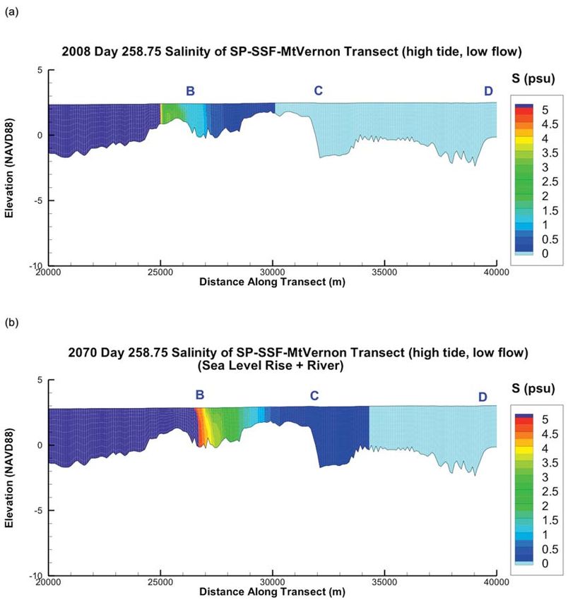
along a longitudinal river transect. Figure 11 Fork (Skagit Wildlife Area). Model predictions
shows a transect (points EDCBA) from Mt. show a notable change in this region with average
Vernon along the South Fork of the Skagit River salinity levels increasing from < 0.5 psu in 2008
to Saratoga Passage. This transect was placed to a higher range from 0.5 to 2 psu for year 2070.
Circulation in the Skagit River Estuary 111Figure 11. Near-shore model grid over the bed, and a selected transect (points EDCBA) though South Fork of Skagit River
for analysis of salinity intruision.
This region of the estuary is part of the Skagit Transport of Skagit River Freshwater Out of
Wildlife Area intertidal marsh complex, which the Estuary
supports valuable salmon habitats. These habitats
could undergo a change from primarily freshwa- Out-migrating salmonids are known to follow
ter (0 to 0.25 psu) to oligohaline (0.5 to 2 psu) the freshwater plume transport pathways and
habitats in the future as a result of SLR. Intrusion brackish water availability at various locations
of saline water further upstream occurs during in the system is an important consideration for
high tide and low river flow. Salinity contour plots habitat restoration planning and design (Beamer
during the high tide in September 2008 (Julian et al 2005a, 2005b). Similarly, an understanding
Day 258.75) and shown in Figure 12. In 2008, of salt water fluxes into the estuary through the
the 0.5 psu salinity contour is shown to extend basin boundaries is also of interest given the
about 1 km upstream of point B as shown in Fig importance of salinity gradients to the estuarine
12(a). The year 2070 simulation shows that the ecosystem and the possibility that the existing
0.5 psu salinity intrusion occurs approximately distribution and transport volumes may be altered
3 km further upstream midway between point C as a result of future climate changes. Using the
near Conway and point B near the tidal marsh results generated, we computed volume fluxes of
region. The influence of future salinity intrusion freshwater and saltwater based on a finite-volume
clearly does not extend beyond confluence of the mass-balance approach for the vertical transects
North and South Forks (point D), which is about as shown in Figure 13. For each transect, the total
12 km downstream of Mt. Vernon. volume flux (total flow rate across a given transect),
112 Khangaonkar et al.Figure 12. Simulated salinity profile along a transect (points EDCBA) for year 2008 (top panel) and 2070 (bottom panel) at
low river flow time (September) and high tide. Color contours were selected such that salinity above 5 psu is in dark
purple (on left) and salinity of 0 psu is in light blue (on right). The 2070 simulation included both SLR and future river
discharge.
and freshwater flux (freshwater component of the through Deception Pass (A-A1) and Swinomish
total flow) were calculated. Channel (B-B1). Estuarine exchange flow enters
A summary of the computed fluxes for years Skagit Bay from the south and was computed at
2008 and 2070 respectively is provided in Table transect C-C1. A portion of Skagit River freshwater
5. The values presented are a year-long average is transported out (due south) from the estuary
of the flux values generated at each transect. The through the surface layers at C-C1, but the net
results show that under exiting conditions, es- volume transport is into the estuary (due north)
tuarine flow is primarily exported from the basin and is dominated by the inflow through the lay-
Circulation in the Skagit River Estuary 113ers below the pycnocline at this location.
This finding also is consistent with results
published by Khangaonkar et al. (2012)
where tidally averaged flow at the C-C1
location showed an outflow through the
shallow brackish surface layer and inflow
into the estuary through the lower layers. In
this study, we used a projected year 2070
hydrograph that included a 13% increase
in the total inflow (Table 1) as reflected in
mean flux through EE1. Mean flux through
transect C-C1, which is a combination of
estuarine exchange flow and freshwater
outflow, increased in 2070 (Table 5). The
total flow out from the estuary appears
to be predominantly through Deception
Pass and is also higher in 2070 relative
to 2008 because of the combined effects
of increased river discharge and estuarine
exchange inflow from Saratoga Passage.
During year 2008, approximately 63%
of the Skagit River flow was carried by the
North Fork while the South Fork carried
the remaining 37%. This distribution is
likely a function of flow magnitude and
Figure 13. Locations of transects A-A1, B-B1, C-C1, D-D1, E-E1, water depth, and the ratio changed to
F-F1, G-G1, H-H1, I-I1 at which the volume fluxes and
salinity fluxes were calculated.
60:40 for the simulated higher flows in
TABLE 5. Simulated total and freshwater flows through the selected transects in Skagit River Estuary for the years 2008 and
2070. The negative values indicate flow direction into the study domain through the respective transects while + sign
indicates flow out of the domain.
Total flow Freshwater component of flow
2008 2070 2008 2070
Mean Flow Mean flow Mean flow Mean flow
Transect (m3/s) (m3/s) (m3/s) (m3/s)
E-E1 (T6)
Skagit River Total -445.4 -503.2 -445.4 -503.2
F-F1 (T7)
North Fork -279.06 -304.5 -279.06 -304.5
G-G1 (T8)
South Fork -166.7 -199.3 -166.7 -199.3
C-C1 (4)
Saratoga Passage -830.6 -834.0 +190.4 +183.3
A-A1 (1)
Deception Pass +1225.9 +1265.4 +303.12 +334.8
B-B1 (3)
Swinomish Channel +75.3 +78.9 +18.8 +21.8
H-H1 (9)
West Pass – Stillaguamish River +0.4 -1.7 -1.7 -6.7
114 Khangaonkar et al.year 2070. Most of the freshwater is exported and lower summer flows will increase salinity in
from the estuary through Deception Pass to the the near-shore environment and result in possible
north and Saratoga Passage to the south and only upstream salinity intrusion. However the results
a small fraction (4%) is transported to Padilla indicate clearly that the magnitude of the changes
Bay through Swinomish Channel. The simulated on the Skagit River estuary is relatively small for
distributions of freshwater transport magnitudes the perturbations considered. The results show that
for the year 2070 simulation are summarized in estuarine circulation and transport subjected to the
Table 6. Freshwater export from Skagit Bay to perturbations described above will result only in
the south through Saratoga Passage decreased, incremental changes to this salinity structure and
and export through Deception Pass increased as inter-basin freshwater distribution and transport,
a result of future conditions. The export of fresh- and none of the simulations showed a dramatic
water from Skagit Bay to Padilla Bay through disruption of estuarine circulation and transport
the Swinomish Channel is predicted to remain in the future.
relatively unchanged based on these test results. The results show that salinity levels at repre-
TABLE 6. Distribution of Skagit River freshwater flow sentative near-shore locations in the future during
through the selected reaches of the estuary. the low-flow summer months are predicted to be
higher (5 1 psu higher for the simulated year 2070
2008 % of 2070 %
Flows Transect Total Flow of Total
conditions). This is primarily due to the predicted
3% increase in exchange flow from Puget Sound-
Skagit River Inflow E-E1 100% 100%
Whidbey Basin and lower river discharge during
North Fork F-F1 63% 61%
South Fork G-G1 37% 40% the summer months for future conditions in year
2070. Salinity intrusion measured using contour
Freshwater Outflow
Deception Pass A-A1 53% 58% resolution of band of 0.5 psu in the future was
Swinomish Channel B-B1 4% 4% detected approximately 3 km further upstream
Saratoga Passage CC1 43% 36% relative to 2008 in the South Fork of Skagit
West Pass to Port Susan H-H1 0% 1% River. Average salinity intrusion is not predicted
to extend beyond Conway, Washington, below
Conclusion the confluence of North Fork and South Fork,
and well downstream of the City of Anacortes
Amid uncertainty associated with projections of
drinking water intake near Mt. Vernon.
future climate and consequent impacts, sensitivity
tests using numerical tools provides a convenient Sufficiently away from the effects of river
way to obtain quantitative information about the plumes, the results show that the mean salinity
relative magnitudes of change that might be ex- levels averaged over a duration of one year are
pected. A synoptic data-collection program with relatively unchanged at all stations in the greater
stations in the interconnected basins of Skagit Bay Salish Sea study domain. Although the effect of
and Padilla Bay allowed development and calibra- SLR on the estuarine exchange is significant,
tion of an embedded high-resolution representa- resulting in nearly 4% increase in marine water
tion of Skagit-Padilla Bay system within SSM. A inflow to Salish Sea, the simulated impact on near-
sensitivity level analysis was conducted using the shore salinity distribution is relatively small. This
model to assess the effects of future (2070) climate is likely because the results presented here assume
change relative to present conditions (2008) in that incoming upwelled Pacific Ocean marine water
the form of SLR (0.46 m) and altered hydrology quality including salinity in year 2070 will be the
(13% higher total flow with 5 80% higher winter same as that observed in year 2008. Our ability
and spring flows and lower summer flows) on to predict future impacts to near-shore salinity
estuarine circulation and transport. The results gradients is therefore dependent and sensitive to
with respect to circulation and estuarine salinity the estimates of quality of Pacific Ocean marine
are in line with the expectation that higher SLR water entering the Salish Sea system in the future.
Circulation in the Skagit River Estuary 115Estuarine exchange flow or volume flux com- These results indicate that the overall structure
putations provided an insight into the transport of oceanographic circulation and transport will
pathways in and out of the Skagit River estuary. likely not be significantly altered as a result of
The results establish a net residual flow of ma- SLR and future flows especially when year-long
rine water through the system with a magnitude average conditions are examined. The overall ef-
5 1.9 times the average river inflow, which travels fect of SLR and hydrological modifications is to
north into Skagit Basin through the Saratoga incrementally strengthen the estuarine transport
Passage. This flow combined with a portion of through the system in the northern direction from
freshwater from the Skagit River exits the basin Saratoga Passage to Deception Pass.
through Deception Pass. The expectation based We do note, however, that the scenarios con-
on examination of fish tracking data collected in sidered only a conservative SLR of 0.46 m and
the basin was that most of freshwater from Skagit hydrology corresponding to moderate emissions
River carrying the out-migrating fish exited the scenario A1B. The simulations also included an ap-
basin toward the north, through the Deception proximation that estuarine inflow into Puget Sound
pass and the Swinomish Channel (Lee et al.
and, therefore the Skagit Basin, will be at same
2010). The results in contrast show that export
salinity in the future. The results therefore should
pathways are comparable through the north and
be treated as preliminary estimates until results
south boundaries through the surface layers. A
from more extensive analyses become available.
little over half (53%) of Skagit River freshwater
is transported out to Puget Sound via Deception Acknowledgments
Pass while a comparable and significant fraction,
nearly 43%, of Skagit River water is transported This work would not have been possible without
south to Saratoga Passage based on existing Year technical input and contributions from our col-
2008 simulations. Only 5 4%, a small fraction leagues from the Skagit Climate Science Consor-
of total freshwater delivered to the Skagit Basin tium. We also acknowledge our collaborators Karol
makes it to Padilla Bay through the Swinomish Erickson and Mindy Roberts from the Washington
Channel. As in the case of the salinity distribu- State Department of Ecology and Ben Cope from
tion, the transport pathways are not significantly the U.S. Environmental Protection Agency for
altered for the future scenarios that we examined. their encouragement and support.
Literature Cited Chinook Salmon in the Greater Skagit River Es-
tuary. Field Sampling and Data Summary Report.
Babson, A. L., M. Kawase, and P. MacCready. 2006. Sea-
Department of the Army Seattle District Corps of
sonal and interannual variability in the circulation
Engineers P.O. Box 3755 Seattle, WA.
of Puget Sound, Washington: A box model study.
Atmosphere-Ocean 44:29-45. Chen C., H. Liu, and R. C. Beardsley. 2003. An unstruc-
Beamer, E., A. McBride, C. Greene, R. Henderson, G. tured, finite-volume, three-dimensional, primitive
Hood, K. Wolf, K. Larsen, C. Rice, and K. Fresh. equation ocean model: application to coastal ocean
2005a. Delta and Nearshore Restoration for the and estuaries. Journal of Atmospheric and Ocean
Recovery of Wild Skagit River Chinook Salmon: Technology 20:159-186.
Linking Estuary Restoration to Wild Chinook Doney, S. C., M. Ruckelshaus, J. E. Duffy, J. P. Barry, F.
Salmon Populations. Appendix D of the Skagit Chan, C. A. English, H. M. Galindo, J. M. Greb-
Chinook Recovery Plan, Skagit River System meier, A. B. Hollowed, N. Knowlton, J. Polovina,
Cooperative, La Conner, WA. N. N. Rabalais, W. J. Sydeman, and L. D. Talley.
Beamer, E., B. Hayman, and D. Smith. 2005b. Linking 2011. Climate change impacts on marine ecosys-
Freshwater Rearing Habitat to Skagit Chinook tems. Annual Review of Marine Science 4:11-37.
Salmon Recovery. Appendix D of the Skagit Chi- Flater, D. 1996. A brief introduction to XTide. Linux
nook Recovery Plan, Skagit River System Coopera- Journal 32:51-57.
tive, La Conner, WA. Foreman, M. G. G., P. Czajko, D. J. Stucchi, and M. Guo.
Beamer, E., C. Rice, R. Henderson, K. Fresh, and M. 2009. A finite volume model simulation for the
Rowse. 2007. Taxonomic Composition of Fish Broughton Archipelago, Canada. Ocean Model-
Assemblages, and Density and Size of Juvenile ing 30:29-47.
116 Khangaonkar et al.Greene, C. M., D. W. Jensen, G. R. Pess, E. A. Steel, and Lee, S-Y., A. F. Hamlet, and E. Grossman. 2016. Impacts
E. Beamer. 2005. Effects of environmental condi- of climate change on regulated streamflow, flood
tions during stream, estuary, and ocean residency control, hydropower production, and sediment
on Chinook salmon return rates in the Skagit River, discharge in the Skagit River basin. Northwest
Washington. Transactions of the American Fisheries Science (this issue).
Society 1562-1581. Mellor, G. L., T. Ezer, and L-Y Oey. 1994. The pressure
Grossman, E. E., A. Stevens, G. Gelfenbaum, and C. Cur- gradient conundrum of sigma coordinate ocean
ran. 2007. Nearshore Circulation and Water Column models. Journal of Atmospheric and Ocean Tech-
Properties in the Skagit River Delta, Northern Puget nology 11:1126-1134.
Sound, Washington—Juvenile Chinook Salmon Mellor, G. L., and T. Yamada. 1982. Development of a
Habitat Availability in the Swinomish Channel. turbulence closure model for geophysical fluid
U.S. Geological Survey Scientific Investigations problems. Review of Geophysics 20:851-875.
Report 2007-5120. Mote, P. W., A. Peterson, H. Shipman, W. S. Reeder, and L.
Hamlet, A. F., S. Y. Lee, N. J. Mantua, E. P. Salathe, A. Whitely Binder. 2008. Sea Level Rise in the Coastal
K. Snover, R. Steed, and I. Tohver. 2010a. Seattle Waters of Washington. Report for the Climate
City Light Climate Change Analysis for the City of Impacts Group, University of Washington, Seattle.
Seattle. Seattle City Light Department, The Climate Mohamedali, T., B. S. Sackmann, and A. Kolosseus.
Impacts Group, Center for Science in the Earth Sys- 2011. Puget Sound dissolved oxygen model: nu-
tem, Joint Institute or the Study of the Atmosphere trient load summary for 1999–2008. Publication
and Ocean, University of Washington, Seattle. No. 11-03-057, Washington State Department of
Hamlet, A. F., P. Carrasco, J. Deems, M. M. Elsner, T. Ecology, Olympia.
Kamstra, C. Lee, S-Y Lee, G. Mauger, E. P. Salathe, National Wildlife Federation. 2007. Sea-level rise and
I. Tohver, and L. Whitely Binder. 2010b. Final coastal habitats in the Pacific Northwest— an analy-
Project Report for the Columbia Basin Climate sis for Puget Sound, southwestern Washington, and
Change Scenarios Project. Climate Impacts Group, northwestern Oregon. Western Natural Resource
Seattle, WA. Center, Seattle, WA.
Hood, W. G. 2006. A conceptual model of depositional, National Research Council. 2011. Climate Stabilization
rather than erosional, tidal channel development in Targets: Emissions, Concentrations and Impacts
the rapidly prograding Skagit River Delta (Washing- over Decades to Millennia. The National Academies
ton, USA). Earth Surface Processes and Landforms Press, Washington, DC.
31:1824-1838. National Research Council. 2012. Sea-Level Rise for the
Khangaonkar, T., Z. Yang, T. Kim, and M. Roberts. 2011. Coasts of California, Oregon, and Washington:
Tidally averaged circulation in Puget Sound sub- Past, Present, and Future. The National Academies
basins: comparison of historical data, analytical Press, Washington, DC.
model, and numerical model. Estuary Coast and Pardaens, A. K., J. M. Gregory, and J. A. Lowe. 2010.
Shelf Science 93:305-319. A model study of factors influencing projections
Khangaonkar, T., and Z. Yang. 2011. A high resolution of sea level over the twenty-first century. Climate
hydrodynamic model of Puget Sound to support Dynamics 36:2015-2033.
nearshore restoration feasibility analysis and design. Rice, C. A. 2007. Evaluting the biological condition of
Ecological Restoration 29:173-184. Puget Sound. Ph.D. Dissertation. University of
Khangaonkar, T., B. Sackmann, W. Long, T. Mohamedali, Washington School of Aquatic and Fishery Sci-
and M. Roberts. 2012. Simulation of annual biogeo- ences, Seattle, WA
chemical cycles of nutrient balance, phytoplankton Roberts, M., T. Mohamedali, B. Sackmann, T. Khanga-
bloom(s), and DO in Puget Sound using an unstruc- onkar, and W. Long. 2014. Dissolved oxygen model
tured grid model. Ocean Dynamics 62:1353-1379. scenarios for Puget Sound and the straits: impacts
Liang, X., D. P. Lettenmaier, E. F. Wood, S. J., and Burges. of current and future nitrogen sources and climate
1994. A simple hydrologically based model of land change through 2070. Publication No. 14-03-007,
surface water and energy fluxes for GSMs. Journal Washington State Department of Ecology, Olympia.
of Geophysical Research 99:14415-14428. Smagorinsky, J. 1963. General circulation experiments with
Lee, C., T. Khangaonkar, Z. Yang, and E. Beamer. 2010. the primitive equations. I. The basic experiment.
Development of a land use planning tool for estua- Monthly Weather Review 91:99-164.
rine habitat protection, restoration, and cumulative Sutherland, D. A., P. MacCready, N. S. Banas, and L. F.
effects assessment in northern Puget Sound, WA. Smedstad. 2011. A model study of the Salish Sea
Report PNWD 4175, prepared for the NOAA/UNH estuarine circulation. Journal of Physical Ocean-
Cooperative Institute for Coastal and Estuarine ography 41:125-1143.
Environmental Technology (CICEET). Batelle Wiggins, W. D., G. P. Ruppert, R. R. Smith, L. L. Reed,
Pacific Northwest Division, Richland, WA. and M. L.Courts. 1997. Water resources data,
Circulation in the Skagit River Estuary 117You can also read