Shrinkage simulation of blow molded parts using viscoelastic material models

Page created by Rhonda Kelly

Science

English

Like
Share
Embed
Fullscreen
Slides
Download HTML
Download PDF
Abuse

←

→

Page content transcription

If your browser does not render page correctly, please read the page content below

Materialwiss. Werkstofftech. 2022, 53, 449–466 doi.org/10.1002/mawe.202100350 449

Shrinkage simulation of blow molded parts using
viscoelastic material models
Schwindungssimulation blasgeformter Bauteile unter
Verwendung viskoelastischer Materialmodelle

P. Michels1, O. Bruch1, 2, B. Evers-Dietze1, D. Grotenburg3,
E. Ramakers-van Dorp1, H. Altenbach4

The utilization of simulation procedures is gaining increasing attention in the prod-
uct development of extrusion blow molded parts. However, some simulation steps,
like the simulation of shrinkage and warpage, are still associated with un-
certainties. The reason for this is on the one hand a lack of standardized inter-
faces for the transfer of simulation data between different simulation tools, and on
the other hand the complex time-, temperature- and process-dependent material
behavior of the used semi crystalline polymers. Using a new vendor neutral inter-
face standard for the data transfer, the shrinkage analysis of a simple blow molded
part is investigated and compared to experimental data. A linear viscoelastic mate-
rial model in combination with an orthotropic process- and temperature-dependent
thermal expansion coefficient is used for the shrinkage prediction. A good agree-
ment is observed. Finally, critical parameters in the simulation models that strongly
influence the shrinkage analysis are identified by a sensitivity study.

Keywords: Linear viscoelasticity / orthotropic process-dependent material behavior /
shrinkage / warpage / integrative simulation / extrusion blow molding

Der Einsatz von Simulationsverfahren gewinnt in der Produktentwicklung extrusions-
blasgeformter Kunststoffhohlkörper zunehmend an Bedeutung. Einige Simulations-
schritte, wie z. B. die Simulation von Schwindung und Verzug, sind jedoch noch mit
Unsicherheiten verbunden. Grund dafür ist zum einen das Fehlen standardisierter
Schnittstellen für den Transfer von Simulationsdaten zwischen verschiedenen Soft-
waretools und zum anderen das komplexe zeit-, temperatur- und prozessabhängige
Materialverhalten der verwendeten teilkristallinen Polymere. Unter Anwendung eines
neuen Schnittstellenstandards für den Datentransfer wird die Schwindungsanalyse ei-
nes einfachen blasgeformten Bauteils untersucht und mit experimentellen Daten ver-
glichen. Für die Schwindungssimulation wird ein linear viskoelastisches Materialmo-
dell in Kombination mit einem orthotropen prozess- und temperaturabhängigen
thermischen Ausdehnungskoeffizienten verwendet. Der Vergleich mit experimentellen
Messdaten zeigt eine gute Übereinstimmung. Abschließend erfolgt eine Sensitivitäts-

1 Bonn-Rhein-Sieg University of Applied Sciences, Corresponding author: P. Michels, Bonn-Rhein-Sieg
TREE Institute, Sankt Augustin, Germany University of Applied Sciences, TREE Institute,
2 Dr. Reinold Hagen Stiftung, Research and Develop- Grantham-Allee 20, 53757, Sankt Augustin, Germany,
ment, Bonn, Germany E-Mail: patrick.michels@h-brs.de
3 Rikutec Germany GmbH & Co. KG, Altenkirchen,
Germany
4 Otto-von-Guericke-University Magdeburg, Institute
of Mechanics, Magdeburg, Germany
This is an open access article under the terms of the Creative Commons Attribution Non-Commercial NoDerivs License, which permits use and distribution in any
medium, provided the original work is properly cited, the use is non-commercial and no modifications or adaptations are made.
© 2022 The Authors. Materialwissenschaft und Werkstofftechnik published by Wiley-VCH GmbH www.wiley-vch.de/home/muw

450 P. Michels Materialwiss. Werkstofftech. 2022, 53, 449–466

studie zur Identifikation der maßgeblichen Einflussgrößen auf die Schwindungssimu-
lation.

Schlüsselwörter: Lineare Viskoelastizität / orthotropes prozessabhängiges
Materialverhalten / Schwindung / Verzug / integrative Simulation /
Extrusionsblasformen

1 Introduction time and the process-related wall thickness dis-
tribution, the local cooling rates as well as the local
The extrusion blow molding process is one of the demolding temperatures can vary considerably. In
most common methods for the production of hollow general, higher demolding temperatures result in
plastic parts like bottles, cans, fuel tanks or large con- higher shrinkage values and vice versa. The cooling
tainers. During the production, a hollow tube, which rate on the other hand influences the level of ther-
is called parison, is extruded. This parison is then in- mal stresses. After demolding, the final shrinkage
flated against the walls of a cooled mold. After a cer- and warpage result from the reduction of thermal
tain cooling time the part solidifies and can be de- stresses and free thermal shrinkage due to further
molded. Due to relatively short cycle times and the cooling in the ambient air.
manufacturability of complex geometries, a high eco- In order to capture the strong influence on the
nomic efficiency of the process is ensured. However, process conditions, the material behavior of the
because of increasing quality standards and competi- used semi crystalline polymers such as e. g. high-
tion with alternative processing methods, the use of density polyethylene (HDPE), needs to be modeled
computer aided engineering (CAE) methods is in- in a broad time and temperature range. In addition,
creasingly gaining attention. process-dependent orthotropic material behavior
Various research groups presented simulation ap- has been observed for extrusion blow molded parts,
proaches for the extrusion blow molding process cov- which needs to be considered [8–10]. Previous
ering the parison creation, inflation, part cooling and studies use isotropic linear viscoelastic material
finally shrinkage and warpage [1–7]. In order to ach- models to cover the time and temperature depend-
ieve a good prediction, all simulation steps involved ence of the material behavior, but neglect the ortho-
must deliver sufficiently accurate results. These re- tropic process-dependent material behavior [1–7].
sults need to be transferred from one analysis step to In addition to the material description of the shrink-
the following ones. Especially if different software age and warpage simulation, the wall thickness dis-
tools are used for the individual simulation steps, the tribution and the temperatures during cooling also
data transfer is often not straightforward. The re- have a significant influence on the shrinkage be-
quired development of customer-specific interfaces havior. Especially the cooling analysis still shows
can be very time-consuming and cost-intensive. potential for improvement. While in practice a lot
For some simulation steps, like the parison in- of attention is paid to the design of the mold cool-
flation or the simulation of typical product tests, the ing, the interaction with the cooled mold is usually
prediction accuracy is already quite good. Never- neglected in the simulation. So far, there are no
theless, when it comes to the prediction of shrink- simulation models in the open literature that con-
age and warpage, there are still uncertainties. One sider the influence of local flow conditions in the
of the major problems is that the part shrinkage is cooling channels on the temperature distribution of
strongly influenced by the process conditions. Dur- the mold.
ing cooling inside the mold, the shrinkage is possi- In this study, an integrative simulation approach
ble only in thickness direction and is prevented in for the shrinkage and warpage prediction of ex-
all other directions because of the sustained blow- trusion blow molded parts is presented. A new ven-
ing pressure (mold constrained) [1]. Therefore, dor neutral interface standard, the so-called VMAP
thermal stresses build up. After demolding, these standard, is used to enhance the data transfer oper-
stresses lead to shape deviations of the final part ations between different sophisticated simulation
(shrinkage and warpage). Depending on the cooling tools [11]. A computational fluid dynamics (CFD)

Materialwiss. Werkstofftech. 2022, 53, 449–466 Shrinkage simulation of blow molded parts 451

simulation of the cooling channels to improve the tween the individual simulation tasks, a large amount
cooling analysis as well as a process-dependent or- of data needs to be exchanged, Figure 1. As different
thotropic material description for the shrinkage and simulation tools like BSIM, Abaqus and AcuSolve
warpage analysis thus extends the simulation work- are used, the data exchange is not straightforward.
flow presented in [7]. For the latter, an isotropic During the VMAP research project, a vendor-neutral
linear viscoelastic material model is used in con- standard for computer aided engineering data storage
junction with an orthotropic process- and temper- was developed to enhance interoperability in virtual
ature-dependent thermal expansion coefficient. Fi- engineering workflows [13]. Using the VMAP stan-
nally, the influence of the individual simulation dard, the cooling simulation and the shrinkage and
stages on the part shrinkage is investigated by a warpage analysis as well as a computational fluid dy-
sensitivity study to identify the most important in- namics analysis of the cooling channels could be suc-
fluencing factors. cessfully integrated into the standard workflow of
blow molded plastic parts [11]. The fact that the in-
formation is always stored in the same data structure
2 Simulation workflow using the VMAP offers a lot more flexibility, even if different simu-
interface standard lation tools are used.

The simulation workflow used in this study consists
of four main steps, Figure 1. The first step is the 3 Investigations
process simulation, which involves the parison crea-
tion, parison manipulation (e. g. spreading or clamp- Based on previous simulative and experimental
ing), and the inflation. Accuform/BSIM Version 2.5, shrinkage investigations, the prediction accuracy of
a finite element-based software tool for the blow the individual simulation steps is investigated using
molding process, is used for the process simulation. the simulation workflow presented in section 2 [7].
The main result is the wall thickness distribution that Also, critical parameters of the simulation models
is used in all of the following analysis steps. Using a will be investigated by a sensitivity study. In the
self-developed interface, the local stretch ratios and following, the experimental database, the simu-
their orientations are determined for each element of lation models and the sensitivity study are dis-
the process simulation mesh [12]. This information is cussed.
necessary in order to define local orthotropic process-
dependent material behavior. Because different mesh-
es are used for the process simulation and the follow- 3.1 Experimental database
ing analysis steps, a mapping routine is required.
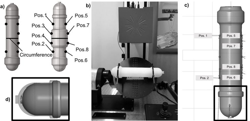
Therefore, the so-called MpCCI mapper of Fraunhof- A cylindrical blow molded part made of the high-
er SCAI is used. Once the process simulation is car- density polyethylene blow molding grade Lupolen
ried out, the cooling of the blown part inside the 5021DX (LyondellBasell) was used for the ex-
closed mold as well as at the ambient air after de- perimental shrinkage measurements in [7], Fig-
molding is analyzed using Simulia/Abaqus. In order ure 2a. Due to the simple geometry and the asso-
to consider the influence of flow-related local heat ciated uniform wall thickness, the part warpage is
transfer coefficients (HTC), a computational fluid dy- minimized, which allows an independent inves-
namics analysis of the cooling channels is carried out tigation of the shrinkage in axial and circum-
using Altair/AcuSolve. The temperature history of the ferential direction. To examine the influence of the
cooling analysis is used in a subsequent thermal me- process conditions, varying wall thicknesses, de-
chanical analysis to determine the shrinkage and war- grees of stretching and cooling times were inves-
page of the part. As with the cooling simulation Aba- tigated, Table 1.
qus is used for the shrinkage and warpage analysis. To measure the shrinkage in axial and circum-
The deformed shape as well as remaining residual ferential direction, the part surface was scanned using
stresses after shrinkage and warpage occurred can be the GOM ATOS 3D scanner, Figure 2b [7]. Several
used as input for following analysis steps like top- balls embedded in the mold provided measurement
load tests, internal pressure tests or drop tests. Be- marks in axial direction, Figure 2a. The shrinkage in

452 P. Michels Materialwiss. Werkstofftech. 2022, 53, 449–466

Figure 1. Simulation workflow for the prediction of shrinkage and warpage of a typical blow molded intermediate bulk contai-
ner (IBC) using the VMAP interface standard for data transfer operations, based on [11].
Bild 1. Simulationsworkflow für die Vorhersage von Schwindung und Verzug am Beispiel eines typischen blasgeformten
Intermediate Bulk Containers (IBC) unter Verwendung des VMAP Interface Standards für den Datentransfer, angelehnt an
[11].

circumferential direction was determined by compar- points using a thermal camera (FLIR ThermaCAM
ing the circumference of a cut in the middle of the SC1000).
scan to the circumference of the mold. For each test Depending on the test point, the shrinkage varies
point, three parts were scanned after a time period of between 1.4 and 3.3 %, Figure 3 [7]. As expected,
six days (processing shrinkage) and six months (post higher demolding temperatures lead to higher
shrinkage), Table 1. Furthermore, the surface temper- shrinkage and vice versa. After six days, the further
ature after demolding was measured over a time peri- increase of shrinkage is rather low. Furthermore,
od of 280 seconds for one part of the first four test the shrinkage of the circumferential direction is al-
ways higher than the shrinkage in axial direction.

Materialwiss. Werkstofftech. 2022, 53, 449–466 Shrinkage simulation of blow molded parts 453

Figure 2. Blow molded part of the shrinkage investigations [7]. Part geometry and measuring points (a), automated scan of
the part surface (b), distance measurement based on the scan (c), comparison between scan and computer-aided design
(CAD) -model (d).
Bild 2. Blasgeformtes Bauteil, welches für die Schwindungsuntersuchungen verwendet wurde [7]. Bauteilgeometrie und
Messpunkte (a), automatisierter Scan der Bauteiloberfläche (b), Abstandsmessung anhand des Scans (c), Vergleich mit dem
Computer-Aided Design (CAD) -Modell (d).

Table 1. Process variations of the shrinkage investiga-
3.2 Simulation models
tions [7].
Tabelle 1. Prozessvariationen der Schwindungsuntersu-
In the following sections, the individual simulation
chungen [7].
stages are discussed in detail.
Test Degree of stret- Thickness Cooling Amount
Point ching [ ] [mm] time [s]
3.2.1 Process simulation
1 1.5 2 30 4
2 1.5 2 60 4 For the process simulation via BSIM, a cylindrical
3 1.5 4 60 4 parison is meshed with triangle membrane ele-
4 1.5 4 90 4 ments. The diameter of the parison and the axial
and circumferential wall thickness profile are se-
5 2.0 2 30 4
lected based on the machine data of the real par-
6 2.0 2 60 4 ison. For the material modeling, the nonlinear vis-
7 2.0 4 60 4 coelastic K-BKZ model is used. Once the process
8 2.0 4 90 4
simulation is finished, the self-developed interface
is used to determine the local degrees of stretching
and their orientations for each element of the proc-
ess simulation mesh [12]. Together with the wall
This can be explained by the fact that the part is thickness distribution, the data is stored in the
stretched mostly in circumferential direction during VMAP file and mapped to the meshes of the fol-
the inflation which leads to a higher molecule ori- lowing analysis steps.
entation in this direction. With increasing stretching
in circumferential direction, the observed ortho-
tropy of the shrinkage increases.

454 P. Michels Materialwiss. Werkstofftech. 2022, 53, 449–466

Figure 3. Results of the experimental shrinkage measurements [7].
Bild 3. Ergebnisse der Schwindungsmessungen [7].

3.2.2 Cooling simulation pendent material parameters [2, 14]. Since there is
currently no material data set for the used material
The cooling simulation is carried out by Abaqus tak- (Lupolen5021DX, LyondellBasell), the temperature-
ing the interaction with the cooled mold into account. dependent material parameters for heat conductivity,
A mixed finite element mesh of triangular and quad- specific heat capacity, and density will be adopted
rangular shell elements with linear shape functions is from literature for a polyethylene [15, 16]. For the
used for the blow molded part. 15 section points are aluminum mold on the other hand, the use of constant
used across the thickness. For the mold, 3D tetrahe- material parameters is justified. Therefore, the materi-
dron elements with linear shape functions are used. al parameters are taken from a data sheet. All boun-
The analysis is performed in three steps. In the first dary conditions are assumed as convective heat trans-
step, the part cools down under mold constraint, so fer conditions in the following form [15]:
that the outer surface of the part interacts with the
cooled mold. The absorbed heat is dissipated through @T
the cooling channels. In the second step, the mold is l ¼ hðT T U Þ, (1)
@n
removed from the analysis. Finally, in the last step
further cooling of the part at ambient air is considered where T is the temperature at the boundary, TU is
until the demolded part reaches room temperature. To the ambient temperature and h is the heat transfer
determine the temperature field with respect to time, coefficient. The ambient temperature after demold-
Fourier’s thermal equation needs to be solved. To ing and the temperature of the blowing air were
solve this partial differential equation, material pa- measured during the experimental measurements
rameters for density, heat conduction, and specific [7]. During the analysis several heat transfer co-
heat capacity as well as initial and boundary con- efficients need to be specified. The determination
ditions need to be specified. An initial temperature is of these coefficients can be quite challenging. Es-
assigned to the blown part and the mold as initial val- pecially the heat transfer between the part and the
ues. Special attention should be paid to the material mold is quite complex. It depends on the material
parameters. Due to strong changes in the material pairing, the surface roughness and the blowing
properties during crystallization, the use of constant pressure [15]. Investigations on extrusion blow
material parameters can lead to inaccuracies when molded polyethylene bottles using an abrasive
used for semi crystalline polymers [14]. The accuracy blasted aluminum mold and blowing pressures be-
of the simulation can be increased by temperature-de- tween 2 and 8 bar suggest a heat transfer co-

Materialwiss. Werkstofftech. 2022, 53, 449–466 Shrinkage simulation of blow molded parts 455

efficient between 600 W m 2 K 1 and 1000 W m 2 3.2.3 Computational fluid dynamics analysis for the
K 1 [17]. For a mold with a smoother surface, high- determination of local heat transfer coefficients
er values of 1300 W m 2 K 1–1800 W m 2 K 1 were
observed [17]. The heat transfer coefficient be- For the computational fluid dynamics analysis of
tween the inner surface of the part and the blowing the cooling channels, Altair/AcuSolve is used. The
air depends on whether the blown air accumulates cooling channel is meshed with tetrahedron ele-
or is continuously exchanged. In the first case, the ments. At the inlet of the channel, a mass flow of
heat transfer is due to free convection whereas in 0.195 kg s 1 that was measured during the shrink-
the second case, the heat transfer is due to forced age experiments is defined. At the outlet, a zero-
convection. After demolding, the part cools further pressure boundary condition is suggested. At the
down due to free convection. In the case of free wall of the cooling channels as well as at the
convection, a value of 10 W m 2 K 1 can be as- blocked outlets (via plug), the velocity is defined as
sumed for the heat transfer at the inner and outer zero (no-slip wall condition), Figure 4. In order to
surface after demolding [1]. Because the heat trans- get the velocity field of the water flow inside the
fer coefficient between the part and the mold is un- channel, the Navier-Stokes equation needs to be
known, it will be determined by reverse engineer- solved. Assuming a turbulent flow, this is asso-
ing using the results of the thermal camera and a ciated with a high computational effort. To reduce
simulation model of the cooling simulation. In ad- the effort a turbulence model, the so-called Spalart-
dition, the heat transfer coefficient between the part Allmaras model is used. The physical properties of
and ambient air as well as between the inner sur- the water and the parameters of the turbulence
face of the part and the blowing air will be de- model were taken from literature [19, 20]. For the
termined by reverse engineering. The heat transfer determination of the local heat transfer coefficients,
coefficient between the cooling channels and the the AcuSolve method of the non-dimensional tem-
water flow can be calculated globally for a turbu- perature (HTC-method 3) is used [21]. This method
lent flow [18]. It can be also determined locally as allows the calculation of the heat transfer co-
a function of the local velocity by a computational efficient using dimensionless parameters, so that an
fluid dynamics analysis. additional thermal simulation is not necessary. Af-
ter the determination, the local heat transfer co-
efficients are saved in a VMAP file and mapped to

Figure 4. Boundary conditions of the computational fluid dynamics analysis.
Bild 4. Randbedingungen der Strömungssimulation.

456 P. Michels Materialwiss. Werkstofftech. 2022, 53, 449–466

the Abaqus mesh of the cooling analysis using the To characterize the viscoelastic properties of the
MpCCI-Mapper. used polyethylene (Lupolen5021DX, LyondellBa-
sell), dynamic mechanical analysis were performed
using blow molded samples, Figure 5 [7]. The sam-
3.2.4 Shrinkage and warpage analysis ples were stamped out of a blow molded square
bottle both in circumferential and axial direction.
Like the cooling simulation, the shrinkage and war- Using the evaluation software Proteus 6.1 of
page analysis is also carried out in 3 steps using Netzsch, master curves were created in the temper-
Abaqus. In the first step (cooling down under mold ature range between – 20 °C and 120 °C for a refer-
constraint), the degrees of freedom of all nodes are ence temperature of 23 °C using the WLF equation
fixed. Because of the change in temperature, ther- for the time-temperature-superposition. In this spe-
mal stresses will build up. In the second step the cific case, the orthotropy of the elastic modulus is
boundary conditions are changed, so that the part rather low, which corresponds to the results of pre-
can shrink freely in step 3 over a time period of six vious studies, Figure 5 [8, 9].
days. To investigate the influence of gravity on the It is therefore assumed that the observed ortho-
shrinkage behavior, a gravity load is applied after tropy in the shrinkage values is mainly due to the
demolding. A quasi static analysis step (Abaqus thermal expansion. Because of the low effect on the
visco step) using nonlinear geometry is used for the elastic modulus, an isotropic linear viscoelastic ma-
shrinkage analysis. Because the same mesh density terial model (general Maxwell model) is used. The
is used for both cooling simulation and shrinkage time dependent relaxation modulus can be de-
analysis, the results of the cooling simulation can scribed as a Prony series as follows:
be directly imported. In case different mesh den-
!
sities are used, the time history of the temperatures X
N � t
�
could be stored as a VMAP file and mapped to the EðtÞ ¼ E0 1 gj � 1 et j
(2)
mesh of the shrinkage analysis using the MpCCI j¼1

mapper.

Figure 5. Results of the dynamic mechanical analysis using blow molded samples, based on [7]. The samples were stam-
ped out of a blow molded square bottle in axial and circumferential direction.
Bild 5. Ergebnisse der dynamisch-mechanischen Analyse an blasgeformten Proben, angelehnt an [7]. Die Probenentnahme
erfolgte aus blasgeformten Vierkantflaschen in Axial- und Umfangsrichtung.

Materialwiss. Werkstofftech. 2022, 53, 449–466 Shrinkage simulation of blow molded parts 457

E0 is the instantaneous Modulus, gj are the Pro- ature [15, 16], the thermal expansion coefficient is
ny parameters, which describe the stiffness ratio of modified based on the experimental shrinkage re-
the j-th network and τj is the relaxation time of the sults, section 3.1. Isotropic behavior is assumed for
j-th network. For the model calibration, the average high temperatures above 120 °C and for a stretch
of all 6 measurements is transferred from the fre- ratio of 1, which means that there is either no
quency to the time domain [7]. The following ap- stretching at all or the stretching in both directions
proximation formula according to [22] is used for is equal. For higher stretch ratios and temperatures
the conversion [7]: below 120 °C, the isotropic coefficient of thermal
expansion is increased by a constant factor in the
1 direction of maximum stretching (circumferential
f ¼ (3) direction CD) and reduced by the same factor in the
2pt
direction of minimum stretching (axial direction
Since it was only possible to evaluate the mate- AD). The shift factor is fitted for a stretch ratio of
rial behavior up to about 120 °C, because the sam- 1.5 and 2.0 to correspond to the orthotropy of the
ples become too soft, the master curve was ex- experimentally investigated shrinkage values, Fig-
trapolated logarithmically to cover the low stiffness ure 6b.
of higher temperatures [7]. 19 Prony parameters are
used in total to cover the time range of the ex-
perimental curve, Figure 6a. The temperature de- 3.3 Sensitivity study
pendence is taken into account by the WLF equa-
tion. Therefore, the WLF parameters are taken over To get a better overview over the influence of the
from the master curve creation. individual simulation steps on the shrinkage and
To link the thermal with the mechanical material warpage of the part and to identify the most im-
behavior, an orthotropic process-dependent thermal portant model parameters, a sensitivity study is car-
expansion coefficient needs to be defined. Starting ried out. The model variations are discussed in the
with an isotropic temperature-dependent thermal following sections.
expansion coefficient for a polyethylene from liter-

Figure 6. Material data for the shrinkage analysis. Comparison between experimental data and Prony series (a), orthotropic
thermal expansion coefficient in axial direction (AD) and circumferential direction (CD) for a stretch ratio (SR) of 1.5 and 2.0
(b). The experimental master curve (a) was obtained from [7].
Bild 6. Materialdaten für die Schwindungsanalyse. Vergleich zwischen experimentellen Daten und Prony-Reihe (a), ortho-
troper Wärmeausdehnungskoeffizient in axialer Richtung (AD) und in Umfangsrichtung (CD) für ein Verstreckverhältnis (SR)
von 1,5 und 2,0 (b). Die experimentelle Masterkurve wurde aus [7] entnommen.

458 P. Michels Materialwiss. Werkstofftech. 2022, 53, 449–466

3.3.1 Variation of the cooling simulation parts made of the polyethylene type Lupolen
5021DX (LyondellBasell). A parametric study of
In the simulation model of the cooling analysis de- the shrinkage behavior based on the viscoelastic
scribed in section 3.2, just the first cooling cycle is material model presented in section 3.2.3 will be
considered. In practice, several cycles are needed carried out to get a better understanding of the
when starting the process or changing the process shrinkage behavior at different process conditions.
conditions to ensure a stable process. Therefore, the For simplification, a one element model consider-
influence of several cycles on the temperature dis- ing isotropic temperature-dependent thermal ex-
tribution of the mold is investigated. Furthermore, pansion will be used in the parametric study. It is
the influence of local heat transfer coefficients of assumed that the cooling rate and the demolding
the cooling channels determined by the computa- temperature are the most important parameters.
tional fluid dynamics simulation presented in sec- Therefore, the shrinkage for a broad range of cool-
tion 2 is compared to a model with a globally con- ing times and cooling rates (different wall thick-
stant heat transfer coefficient. Also, a cooling nesses) is investigated.
simulation without mold interaction will be carried
out. In this case the heat transfer coefficient be-
tween the part and the mold will be used with a 4 Results and discussion
globally constant steady-state temperature. Finally,
the influence of the heat transfer coefficient be- In the following, the results of the simulation mod-
tween the blown part and the mold will be inves- els will be compared to the experimental measure-
tigated. For simplification, the isotropic temper- ment data and the outcome of the sensitivity study
ature dependent thermal expansion coefficient will be discussed.
according to [15, 16] is used. The influence is in-
vestigated for the first four test points of the shrink-
age experiments, Table 1. 4.1 Simulation results

The results of the process simulation for 2 mm and
3.3.2 Variation of the process simulation 4 mm wall thickness are compared to experimental
data of the first four test points, Figure 7. For the
The prediction accuracy of the process simulation thickness measurement, the parts were cut in half.
strongly depends on the geometry of the part and The GOM ATOS 3D scanner was used to scan the
the experience of the user. In many cases, an accu- inner and outer surface of the half in order to de-
racy between 80 %–90 % or even more can be ach- termine the thickness. Using the MpCCI mapper
ieved. In order to estimate the influence of an error the measured wall thickness distribution was map-
of the wall thickness on the part shrinkage, the in- ped to the simulation mesh in order to visualize the
fluence of + / 10 % error in thickness prediction percentage deviation between the measurements
is investigated. A one-element-model using the lin- and the process simulation. Even if there are larger
ear viscoelastic model described in section 3.2.4 is deviations in partial areas, the deviation in the area
used in conjunction with the isotropic temperature- in which the shrinkage measurement was carried
dependent thermal expansion coefficient. out (square) is mostly below 5 %, Figure 7.
The results of the computational fluid dynamics
simulation illustrate the strong dependence of the
3.3.3 Shrinkage and warpage analysis heat transfer coefficients on the local flow con-
ditions, Figure 8. In the backwater areas (dark
The experimental shrinkage investigations refer to areas) the velocity is zero. The average velocity is
specific points in time, six days and six months af- about 5 m s 1 that leads to a heat transfer co-
ter demolding. Once the part is demolded, the ther- efficient of about 24000 W m 2 K 1. In some areas
mal stresses result in creep behavior of the part the local heat transfer coefficients are even higher
[23]. So far, the dynamic creep behavior after de- than 40000 W m 2 K 1. This is a big difference to
molding has not been investigated for blow molded the global coefficient, which has been calculated

Materialwiss. Werkstofftech. 2022, 53, 449–466 Shrinkage simulation of blow molded parts 459

Figure 7. Percentage deviation of the wall thickness simulation from the measured components of test points (TP) 1, 2, 3
and 4, Table 1.
Bild 7. Prozentuale Abweichung der Wanddickensimulation von den vermessenen Bauteilen der Versuchspunkte (TP) 1, 2,
3 und 4, Tabelle 1.

Figure 8. Results of the computational fluid dynamics analysis. Velocity (a), local heat transfer coefficients (HTC) (b) and
local heat transfer coefficients (HTC) mapped to the Abaqus mesh of the cooling analysis (c).
Bild 8. Ergebnisse der Strömungssimulation. Geschwindigkeitsfeld (a), lokale Wärmeübergangskoeffizienten (HTC) (b) und
auf das Netz der Abkühlsimulation gemappte Wärmeübergangskoeffizienten (HTC) (c).

with 9370 W m 2 K 1. A comparison between the thermal measurements in the middle area of the
globally determined heat transfer coefficient and blown part for the first four test points, Figure 9.
the local heat transfer coefficients of the computa- Because the measurement of the temperatures while
tional fluid dynamics analysis will be discussed in the part is still in the mold is quite difficult, the
section 4.2. temperatures of the outer surface after demolding
The results of the cooling analysis using the lo- were measured by a thermal camera for a period of
cal heat transfer coefficients are compared to the 280 seconds [7]. Due to the fitted heat transfer co-

460 P. Michels Materialwiss. Werkstofftech. 2022, 53, 449–466

The stretch ratio in the middle area, where the
shrinkage measurements took place, is about 1.5 for
the test points 1–4 and about 2.0 for the test points
5–8, Figure 10. The maximum stretching is ori-
ented mostly in circumferential direction, whereas
the minimum stretching is oriented mostly in axial
direction.
Using the orthotropic thermal expansion co-
efficient, the simulation is able to match the level
of orthotropy observed in the experiments, Fig-
ure 11. However, the shrinkage is a little bit under-
predicted by the simulation. In addition, the simu-
lation is not able to capture the qualitative
shrinkage behavior of the test points 1, 2 and 4 as
well as 5, 6 and 8. A comparison of the simulation
models with and without gravity shows that the in-
fluence of gravity is negligible. This result is in
contrast to warpage investigations of previous stud-
ies on blow molded automotive parts [2, 3]. How-
Figure 9. Comparison between the cooling analysis and the
thermal camera image for the test points (TP) 1, 2, 3 and 4,
ever, the parts investigated in these studies have a
Table 1. The measurement data were taken from [7]. very long and thin shape and seem to be subject to
Bild 9. Vergleich zwischen der Abkühlsimulation und dem high warpage. It is therefore assumed that the influ-
Ergebnis der Thermokamera für die Versuchspunkte (TP) 1, ence of gravity depends on the geometry of the
2, 3 und 4, Tabelle 1. Die Messdaten wurden aus [7] ent- part.
nommen.

4.2 Model variations
efficients (section 3.2.2), the simulation results are
in good agreement with the experimental measure- For the simulation results presented in section 4.1,
ments. The biggest deviation shows test point 1. just the first cooling cycle was considered. After

Figure 10. Illustration of the determined stretch ratios of the test points (TP) 1, 3, 5 and 7, Table 1.
Bild 10. Darstellung der ermittelten Verstreckgradverhältnisse für die Versuchspunkte (TP) 1, 3, 5 und 7, Tabelle 1.

Materialwiss. Werkstofftech. 2022, 53, 449–466 Shrinkage simulation of blow molded parts 461

Figure 11. Comparison between the shrinkage analysis and experimental shrinkage measurements. The measurement
data were taken from [7].
Bild 11. Gegenüberstellung der Simulationsergebnisse mit den experimentellen Schwindungswerten. Die Messdaten wur-
den aus [7] entnommen.

seven cycles the mold has heated up, Figure 12. molding temperature is less than 1 °C lower than
However, the difference in temperature is quite the demolding temperature by the use of global
small. It can be concluded that after about five cy- heat transfer coefficients, Figure 14a. Con-
cles, an equilibrium state is reached, Figure 13. The sequently, the influence on shrinkage is also very
seventh cycle is compared to measurement data of low, Figure 14b. The reason for this could be that
thermocouples, which were placed in different the distance between the cooling channels and the
areas close to the cavity. The simulated mold tem- cavity is rather high. Furthermore, the global heat
perature is thus a little underestimated. Because of transfer coefficient itself is already quite high, so
the temperature-dependent material parameter and that a further increase has probably just a small ef-
the high cooling rates at the outer surface, the com- fect. Even the model without mold interaction and
putation time of the cooling analysis is quite high also a simplified one element model lead to quite
(about 7 h for each cycle using ten cores of an good results. The average mold temperature of the
AMD Ryzen9 3900X). Considering the small measurements was used for the model without
changes in the mold temperatures, the simulation of mold interaction and the one element model. In the
the first cycle is considered as sufficient for this case of this special component, the consideration of
specific model. the local heat transfer coefficients of the cooling
To evaluate the influence of the local heat trans- channels and even the mold interaction in general
fer coefficients of the cooling channels and the in- seems to play a rather subordinate role. However,
fluence of the mold interaction in general, the de- for complex blow molded parts with cooling chan-
molding temperature and the resulting shrinkage nels close to the cavity, it cannot be ruled out that
was evaluated for an element in the middle of the the mold cooling system has a significant influence
simulation model. Because of the high thermal gra- on the local demolding temperatures. At this point,
dient in thickness direction, the demolding temper- further investigations at complex blow molded
ature was determined by taking the average of all parts are necessary.
15 section points across the part thickness. The in- In contrast to the local heat transfer coefficient
fluence of the local heat transfer coefficients of the of the cooling channels, the heat transfer coefficient
cooling channels is rather low. The average de- between the blown part and the mold is of high im-

462 P. Michels Materialwiss. Werkstofftech. 2022, 53, 449–466

Figure 12. Comparison of the mold temperature of test
point 2 after the first (a) and the seventh cycle (b).
Bild 12. Gegenüberstellung der Temperaturverteilung der
Werkzeugform von Versuchspunkt 2 nach 1 Kühlzyklus (a)
und 7 Kühlzyklen (b).

portance, Figure 15. For the simulation models pre- Figure 13. Comparison of the first 7 cooling cycles of test
sented in section 4.1, the heat transfer coefficient point 2 to experimental measurement data at two different
positions (T1 and T2). The temperature sensors were pla-
has been determined by reverse engineering with a ced in the upper area (a) and in the middle of the component
value of about 1000 W m 2 K 1. As discussed in (b). The experimental measurement was carried out after
section 3, it depends considerably on the blowing the system had reached a steady state and is compared to
pressure, the roughness of the surface, and the ma- the seventh cycle of the simulation.
terial pairing. According to the investigations in Bild 13. Vergleich der ersten 7 Kühlzyklen von Versuchs-
punkt 2 mit experimentellen Messdaten an zwei verschiede-
[17], it seems reasonable to vary the heat transfer nen Temperaturfühlerpositionen (T1 und T2). Die Tempera-
coefficient between 600 W m 2 K 1 and turfühler wurden dafür im oberen Bereich (a) und in der Mitte
2 1
1800 W m K . Depending on the test point, the des Bauteils (b) platziert. Die experimentelle Messung wur-
change in the average demolding temperature based de erst durchgeführt, nachdem das System einen stabilen
on the initial heat transfer coefficient of about Zustand erreicht hatte. Der Vergleich erfolgt mit dem siebten
Zyklus der Simulation.

Materialwiss. Werkstofftech. 2022, 53, 449–466 Shrinkage simulation of blow molded parts 463

Figure 14. Variation of the cooling analysis. Influence on
the average demolding temperature (a) and influence on the
part shrinkage (b). Figure 15. Variation of heat transfer coefficient between the
blown part and the mold. Influence on the average demolding
Bild 14. Variation der Abkühlsimulation. Einfluss auf die ge-
temperature (a) and influence on the part shrinkage (b).
mittelte Entformungstemperatur (a) und Einfluss auf die
Bauteilschwindung (b). Bild 15. Variation des Wärmeübergangskoeffizienten zwi-
schen Artikel und Blasformwerkzeug. Einfluss auf die gemit-
telte Entformungstemperatur (a) und Einfluss auf die Bau-
teilschwindung (b).
1000 W m 2 K 1 varies between 6 and 37 %, Fig-
ure 15a. The effect on the shrinkage is up to 17 %
(test point 1), Figure 15b. Due to its great influ- ure 16. The change based on the initial wall thick-
ence, the heat transfer coefficient between the part ness is in the range of 6 %–28 % for the demolding
and the mold should be examined more closely for temperature and in the range of 0 %–24 % for the
varying surface roughness and blowing pressures. shrinkage, depending on the test point. In contrast
The wall thickness variation of + / 10 % has to the heat transfer coefficient, whose influence
also a large influence on the average demolding could be reduced through extensive experimental
temperature and the resulting part shrinkage, Fig- investigations, errors in the wall thickness dis-

464   P. Michels                                                                                   Materialwiss. Werkstofftech. 2022, 53, 449–466

                                                                                   sults allow an insight in the shrinkage behavior
                                                                                   with respect to the average demolding temperature,
                                                                                   Figure 17. The shrinkage values six days after de-
                                                                                   molding are illustrated as functions of the average
                                                                                   demolding temperature for several thickness values,
                                                                                   Figure 17a. The simulation results of the four test
                                                                                   points are marked by the circles. It is clearly visible
                                                                                   that at temperatures of approx. 90 °C, the relation-
                                                                                   ships are inverted. While low wall thicknesses
                                                                                   show lower shrinkage at temperatures above 90 °C,
                                                                                   they show higher shrinkage at temperatures below
                                                                                   90 °C. At low demolding temperatures, higher re-
                                                                                   sidual stresses occur in thin wall thicknesses due to
                                                                                   faster cooling. For high demolding temperatures on
                                                                                   the other hand, the cooling at ambient air is much
                                                                                   slower for high wall thicknesses, so that residual
                                                                                   stresses have more time at high temperatures to re-
                                                                                   lax.
                                                                                       In addition, the shrinkage for 2 mm thickness is
                                                                                   illustrated for different periods, Figure 17b. For
                                                                                   temperatures above 50 °C, there is no further in-
                                                                                   crease in shrinkage after one hour past demolding.
                                                                                   In this case, very long creep times would be neces-
                                                                                   sary for a further increase in shrinkage. For lower
                                                                                   temperatures, a strong creep behavior is observed,
                                                                                   which diminishes with increasing time. Un-
                                                                                   fortunately, an experimental database is lacking for
                                                                                   a conclusive evaluation of the observed effects.

                                                                                   5 Conclusions

                                                                                   In this work, a simulation workflow for the pre-
                                                                                   diction of shrinkage and warpage of extrusion blow
                                                                                   molded plastic parts is presented. The VMAP inter-
                                                                                   face standard is used for the data transfer between
      Figure 16. Variation of the wall thickness. Influence on the
      average demolding temperature (a) and influence on the
                                                                                   the different software tools that are used within the
      part shrinkage (b).                                                          workflow. For the cooling analysis, the interaction
      Bild 16. Variation der Wanddicke. Einfluss auf die gemittel-                 of the blown part and the cooled mold is consid-
      te Entformungstemperatur (a) und Einfluss auf die Bauteil-                   ered. Local heat transfer coefficients, which were
      schwindung (b).                                                              determined by a subsequent computational fluid dy-
                                                                                   namics analysis, are used for the heat dissipation at
                                                                                   the cooling channels. A linear viscoelastic material
      tribution can hardly be avoided. Thus, one should                            model in combination with an orthotropic process-
      be aware of this possible error when designing                               and temperature-dependent thermal expansion co-
      blow molded parts.                                                           efficient is used to capture the complex material be-
          Finally, in a parametric study, the shrinkage be-                        havior of the semi crystalline polymer poly-
      havior by the use of the linear viscoelastic material                        ethylene. While the orthotropy of the shrinkage is
      model has been investigated for several wall thick-                          already well predicted, the simulation results de-
      nesses and a broad range of cooling times. The re-

      © 2022 The Authors. Materialwissenschaft und Werkstofftechnik published by Wiley-VCH GmbH                         www.wiley-vch.de/home/muw

Materialwiss. Werkstofftech. 2022, 53, 449–466 Shrinkage simulation of blow molded parts 465

Figure 17. Simulated shrinkage values with respect to the average demolding temperature. Comparison of different wall
thicknesses (a) and comparison of the shrinkage for 2 mm wall thickness for different points in time after demolding (b).
Bild 17. Simulierte Schwindungswerte in Abhängigkeit von der gemittelten Entformungstemperatur. Vergleich verschiedener
Wandstärken (a) und Vergleich der Schwindung für 2 mm Wandstärke zu verschiedenen Zeitpunkten nach der Entformung
(b).

viate from the measured values both qualitatively amine the component warpage due to differences in
and quantitatively. the local shrinkage.
In a sensitivity study, the influence of the in-
dividual simulation stages was investigated. The
heat transfer coefficient between the blown part and Acknowledgements
the mold as well as errors in the wall thickness sim-
ulation show the biggest influence on the part This work was funded by the German Federal Min-
shrinkage. The influence of the local heat transfer istry of Education and Research (BMBF) via the
coefficients determined by the computational fluid ITEA3 cluster of the European research initiative
dynamics simulation as well as the simulation of EUREKA (Funding Sign BMBF 01 j S17025A–K).
several cooling cycles shows a rather small influ- We would also like to thank the Graduate Institute
ence. Furthermore, in a parametric study, the and the TREE Institute of Hochschule Bonn-Rhein-
shrinkage behavior has been investigated for a huge Sieg University of Applied Sciences for their finan-
range of demolding temperatures and wall thick- cial support. Open access funding enabled and or-
nesses. Based on the results, it is clearly visible that ganized by Projekt DEAL.
the selected test points are not well chosen to inves-
tigate the highly nonlinear shrinkage behavior of
blow molded parts. Additional shrinkage inves- 6 References
tigations at different wall thicknesses and several
demolding temperatures are necessary to evaluate [1] D. Laroche, K.K. Kabenemi, L. Pecora, R.W.
the prediction accuracy of the used material model. DiRaddo, Polym. Eng. Sci. 1999, 39, 1223.
Therefore, the cooling and the shrinkage behavior [2] P. Debergue, H. Massé, F. Thibault, R.
should be examined as comprehensively as possi- DiRaddo, presented at 6th ESAFORM Confer-
ble. A dynamic shrinkage measurement immedi- ence on Material Forming, Salerno, Italy,
ately after demolding as well as measurement at April 28–April 30, 2003, pp. 23–26.
different points in time could provide valuable in- [3] P. Debergue, H. Massé, F. Thibault, R.
formation. In addition, more complex blow molded
DiRaddo, SAE Trans. 2003, 112, 359.
components should be investigated in order to ex-

466   P. Michels                                                                                   Materialwiss. Werkstofftech. 2022, 53, 449–466

       [4] Z. Benrabah, P. Debergue, R. DiRaddo, SAE                                      perability 2020, Virtual Conference, October
           Trans. 2006, 115, 493.                                                         19- October 20, 2020, pp. 11–16.
       [5] Z. Benrabah, H. Mir, Y. Zhang, SAE Int. J.                              [14]   W. Michaeli, P. Niggemeier, Kunststoffe
           Mater. Manuf. 2013, 6, 349.                                                    1999, 89, 70.
       [6] Z. Benrabah, A. Bardetti, F. Ilinca, G. Ward,                           [15]   A. Kipping, Ph.D. Thesis, University Siegen,
           presented at ANTEC 2018 Conference, Orlan-                                     Germany, 2004.
           do, USA, May 7- May 10, 2018, pp. 2635–                                 [16]   VDMA, Thermodynamik. Kenndaten für die
           2643.                                                                          Verarbeitung thermoplastischer Kunststoffe
       [7] P. Michels, O. Bruch, B. Evers-Dietze, E.                                      Teil 1, Hanser, München, 1979.
           Ramakers-van Dorp, H. Altenbach, presented                              [17]   H.G. Speuser, Ph.D. Thesis, RWTH Aachen,
           at 14. Magdeburger Maschinenbautage, Sep-                                      Germany, 1992.
           tember 24–September 25, 2019, pp. 198–208.                              [18]   V. Gnielinski, Wärmeübertragung bei der
       [8] D. Grommes, O. Bruch, J. Geilen, AIP                                           Strömung durch Rohre, VDI-Wärmeatlas -
           Conference Proceedings 2016, 1779, 50013.                                      Chapter Ga, Springer, Berlin, Heidelberg,
       [9] E. Ramakers-van Dorp, C. Blume, T. Hae-                                        2006.
           decke, V. Pata, D. Reith, O. Bruch, B.                                  [19]   W. Wagner, H.J. Kretzschmar, VDI-Wärmeat-
           Möginger, V. Hausnerova, Polym. Test. 2020,                                    las - Chapter D2, Springer, Berlin, Heidel-
           77, 105903.                                                                    berg, Wiesbaden, 2013.
      [10] E. Ramakers-van Dorp, B. Möginger, V.                                   [20]   R. Schwarze, CFD-Modellierung - Grundla-
           Hausnerova, Polymer 2019, 191, 122249.                                         gen und Anwendungen bei Strömungsprozes-
      [11] O. Bruch, P. Michels, D. Grotenburg, pre-                                      sen, Springer, Berlin, Heidelberg, New York,
           sented at the 1st International Conference on                                  2013.
           CAE Interoperability 2020, Virtual Confer-                              [21]   Altair Engineering Inc., AcuSolve Programs
           ence, October 19- October 20, 2020, pp. 103–                                   Reference Manual, 2019.
           105.                                                                    [22]   W. Sommer, Kolloid Z. 1959, 167, 97.
      [12] P. Michels, D. Grommes, A. Oeckerath, D.                                [23]   W. Kulik, Ph.D. Thesis, RWTH Aachen,
           Reith, O. Bruch, Finite Elem. Anal. Des.                                       Germany, 1974.
           2019, 164, 69.
      [13] K. Wolf, P. Gulati, G. Duffett, presented at
           1st International Conference on CAE Intero-                             Received in final form: February 11th 2022

      © 2022 The Authors. Materialwissenschaft und Werkstofftechnik published by Wiley-VCH GmbH                         www.wiley-vch.de/home/muw

You can also read