SIBAR: A NEW METHOD FOR BACKGROUND QUANTIFICATION AND REMOVAL FROM MOBILE AIR POLLUTION MEASUREMENTS
←
→
Page content transcription
If your browser does not render page correctly, please read the page content below
Atmos. Meas. Tech., 14, 5809–5821, 2021
https://doi.org/10.5194/amt-14-5809-2021
© Author(s) 2021. This work is distributed under
the Creative Commons Attribution 4.0 License.

SIBaR: a new method for background quantification and removal
from mobile air pollution measurements
Blake Actkinson1 , Katherine Ensor2 , and Robert J. Griffin1,3
1 Department of Civil and Environmental Engineering, Rice University, Houston, TX 77005, USA
2 Department of Statistics, Rice University, Houston, TX 77005, USA
3 Department of Chemical and Biomolecular Engineering, Rice University, Houston, TX 77005, USA

Correspondence: Robert J. Griffin (rob.griffin@rice.edu)

Received: 14 January 2021 – Discussion started: 28 January 2021
Revised: 24 June 2021 – Accepted: 12 July 2021 – Published: 26 August 2021

Abstract. Mobile monitoring is becoming increasingly pop-        1   Introduction
ular for characterizing air pollution on fine spatial scales.
In identifying local source contributions to measured pollu-
tant concentrations, the detection and quantification of back-   Understanding air pollution exposure is important, as it has
ground are key steps in many mobile monitoring studies,          been linked to various adverse health conditions (Caplin et
but the methodology to do so requires further development        al., 2019; Zhang et al., 2018). Mobile monitoring, a tech-
to improve replicability. Here we discuss a new method for       nique in which continuous air pollution measurements are
quantifying and removing background in mobile monitoring         collected using instrumentation on a mobile platform, is be-
studies, State-Informed Background Removal (SIBaR). The          coming increasingly important for characterizing exposure
method employs hidden Markov models (HMMs), a popu-              because air pollution varies on spatial scales finer than the
lar modeling technique that detects regime changes in time       typical distance between stationary monitors (Apte et al.,
series. We discuss the development of SIBaR and assess its       2017; Chambliss et al., 2020; Messier et al., 2018).
performance on an external dataset. We find 83 % agree-             A key component of mobile monitoring analysis is identi-
ment between the predictions made by SIBaR and the pre-          fying ambient background levels, defined here as measured
determined allocation of background and non-background           air pollution concentrations independent of local source in-
data points. We then assess its application to a dataset col-    fluences (Brantley et al., 2014). Background quantification
lected in Houston by mapping the fraction of points des-         is vital from both policy and exposure perspectives, as it
ignated as background and comparing source contributions         is important to assess the contribution of local sources to
to those derived using other published background detection      pollution concentrations accurately. Table 1 summarizes the
and removal techniques. The presented results suggest that       wide variety of methods used to estimate background in stud-
the SIBaR-modeled source contributions contain source in-        ies incorporating mobile monitoring published within the
fluences left undetected by other techniques, but that they      past 5 years. The wide variance in the approaches used is
are prone to unrealistic source contribution estimates when      problematic, as estimates of source contributions to mea-
they extrapolate. Results suggest that SIBaR could serve as a    surements have been shown to be sensitive to the technique
framework for improved background quantification and re-         used (Brantley et al., 2014). To improve the replicability and
moval in future mobile monitoring studies while ensuring         power of mobile monitoring studies, a more consistent tech-
that cases of extrapolation are appropriately addressed.         nique for background estimation is needed.
                                                                    Designing a method to determine the background in mo-
                                                                 bile monitoring studies presents several challenges. Measure-
                                                                 ments in remote locations are often regarded as the most
                                                                 reliable representation of background concentrations; how-
                                                                 ever, remote locations may be inaccessible for some mobile

Published by Copernicus Publications on behalf of the European Geosciences Union.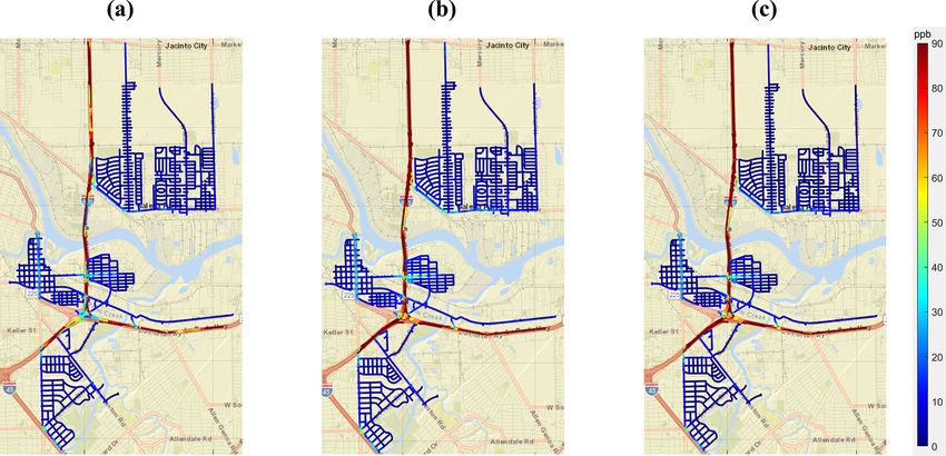
5810                                  B. Actkinson et al.: SIBaR: a new method for background quantification and removal

Table 1. Summary of previous methodologies for estimating background levels of air pollution in mobile monitoring campaigns.

         Study                           Method used to determine background concentration
         Apte et al. (2017)              Applied 10 s moving average filter, then selected the smaller of the given data value or
                                         the 2 min 5th percentile to derive baseline concentrations.
         Brantley et al. (2019)          Fitted quantile regression with cubic natural spline basis expansion of time with degrees
                                         of freedom equal to the number of hours in the time series.
         Hankey and Marshall (2015)      Used pollutant-specific underwrite functions to estimate instantaneous background con-
                                         centrations and subtracted these concentrations from the original time series, averaged
                                         reference monitor measurements, then added averaged measurements to underwrite ad-
                                         justed time series.
         Hankey et al. (2019)            Used hourly averaged measurements in centrally located site for additive correction
                                         factor; used daily median fixed-site measurement for temporal correction factor.
         Hudda et al. (2014)             Applied rolling 30 s 5th percentile of the original time series.
         Larson et al. (2017)            Applied 10 min rolling minimum.
         Li et al. (2019)                Applied 1 min moving median filter, then calculated 1 h rolling 5th percentile of
                                         smoothed data; additionally, used wavelet decomposition to isolate concentration
                                         changes across 8 h at stationary monitors, then subtracted lowest decoupled concen-
                                         tration from mobile monitoring time series across 15 min time windows.
         Patton et al. (2014)            Used mobile measurements in designated urban background neighborhoods removed
                                         from highway.
         Robinson et al. (2018)          Linearly interpolated averaged data collected at designated background locations.
         Shairsingh et al. (2018)        Applied rolling 60 s mean, then applied spline of minimums technique (Brantley et al.,
                                         2014) across different time windows dependent on a desired background scale.
         Tessum et al. (2018)            Used daily 5th percentile for all pollutants other than fine-particle number concentra-
                                         tion; used rolling 30 min 5th percentile for fine-particle number concentration.
         Van den Bossche et al. (2015)   Used averaged measurements from stationary monitor located in an urban green to
                                         apply additive correction factors to measurements greater than background, then av-
                                         eraged site measurement and multiplicative correction factors to measurements lower
                                         than background.

monitoring studies and are themselves subject to occasional             ety of contexts in signals processing, finance, and the social
source influences. These drawbacks make time series meth-               sciences and that has been used to model background in sta-
ods for determining background more desirable. However,                 tionary monitors (Gómez-Losada et al., 2016, 2018, 2019;
many time-series-based methods often rely on setting static             Visser and Speekenbrink, 2010). HMMs assume that obser-
time windows, which are usually determined by the expected              vations within a time series are drawn from probability distri-
duration of influence from source plumes within the mobile              butions governed by a hidden sequence of states. We propose
monitoring study (Bukowiecki et al., 2002). The underlying              decoding this hidden sequence of states as a way to deter-
physical representation of these time series methods remains            mine whether measurements were taken during time periods
unclear for more extensive mobile monitoring campaigns, as              representative of background versus time periods subject to
the setting of static time windows does not often capture the           local influences. We illustrate that a more physically mean-
entire variation in timescales that source impacts can have on          ingful representation of background is captured in this mod-
mobile measurements.                                                    eling context for mobile monitoring time series and show its
   Here we show the results of a newly developed method                 application to a wide variety of traffic-related air pollutant
called State-Informed Background Removal (SIBaR) used to                measurements. As a proof of concept, we run the method on
estimate background for several traffic-related air pollutants,         a published external dataset already marked as background
namely nitrogen oxides (NOx ) and carbon dioxide (CO2 ).                and non-background and assess its performance. As a first
The method incorporates hidden Markov models (HMMs),                    application and to provide further proof of concept, we map
a time series regime modeling technique used in a wide vari-            points binned as background by SIBaR to show their spatial

Atmos. Meas. Tech., 14, 5809–5821, 2021                                                    https://doi.org/10.5194/amt-14-5809-2021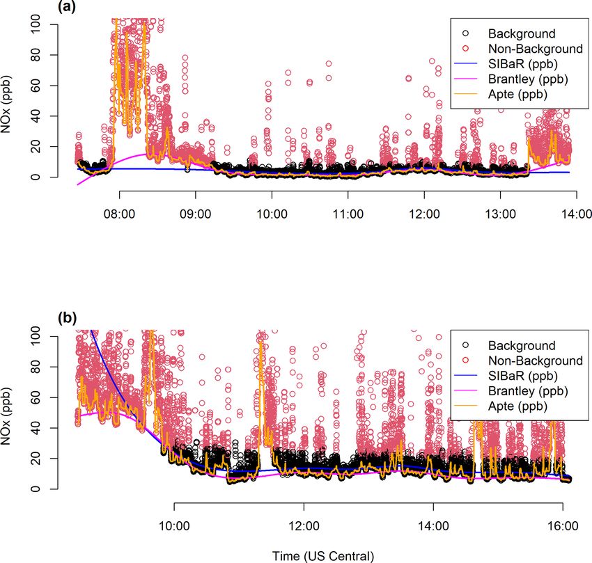
B. Actkinson et al.: SIBaR: a new method for background quantification and removal                                               5811

distributions. As a proof of importance, we highlight differ-       of the study to match the manufacturer reported value. Pre-
ences in mapped source contributions derived from SIBaR             cision values for the T200 and T500U were calculated as the
background and background derived from other time-series-           standard deviation of zeroing periods taken throughout the
based techniques. Results indicate that our consistent method       entire campaign. Minimum detection limits for the T200 and
for background identification and removal has a noticeable          T500U were determined as the mean of the time series zero
impact on mapped mobile source contributions.                       +3σ . The minimum detection limit and precision of the Li-
                                                                    COR were not considered due to taking measurements at a
                                                                    consistently elevated global background and the latter man-
2     Methods                                                       ufacturer’s reported value having a minuscule effect on the
                                                                    overall uncertainty of the measurement. For the purposes of
2.1    Mobile campaign                                              this work, we perform no MDL substitution, as MDL sub-
                                                                    stitution would censor the underlying modeled background
Measurements were taken during the Houston Mobile Mon-              probability distribution.
itoring Google Street View (GSV) campaign and are de-
scribed in detail elsewhere (Miller et al., 2020). Measure-         2.2    Hidden Markov model categorization – the
ments were conducted over a 9 month period spanning July                   background partitioning step
2017 to March 2018. Sampling primarily took place between
07:00 and 16:00 local standard time (Miller et al., 2020) in        Time series observations are segregated by day and for each
a variety of census tracts across metropolitan Houston. Cen-        GSV car, and HMMs are fit to each day’s worth of data. Be-
sus tracts are included in the current analysis if they were        fore fitting the HMM to each day’s time series realizations,
sampled a minimum of 15 times during this 9-month period            we log transform them. HMMs attempt to maximize the log-
(Apte et al., 2017; Li et al., 2019). Details and names used to     likelihood, LC , determined by the sum of the forward vari-
describe each census tract are given in Table S1 in the Sup-        ables αT (i):
plement. The time of day and day of week for each census                   N
                                                                           X
tract visit were predetermined to minimize temporal biases          LC =         αT (i)                                            (1)
in sampling to the greatest extent possible. Instruments (Ta-                i
ble S2) were loaded into two gasoline-powered GSV cars that         in which i designates state i (total states N) at the last realiza-
sampled every drivable road in 22 different census tracts in        tion of the time series T . The forward variables are derived
the greater Houston area. Details and names used to describe        recursively as
each of the census tracts considered are given in Table S1. In-
dividual observations are aggregated to 50 m points in neigh-       α1 (i) = πi p (y1 |θi , z)                                     (2)
                                                                                XN
borhoods and 90 m points on highways using a road network           αt+1 (j ) =         α    (i)a

                                                                                                       p y  |θ  , z

                                                                                                                                   (3)
                                                                                    i      t      ij      t   j
created from U.S. Census TIGER/Line roads (TIGER/Line
Shapefile, 2018). More details on the road network creation         in which πi represents the initial probability for state i, aij
and data quality control are provided elsewhere (Miller et          represents the state transition probability from state i to state
al., 2020). Data quality and control measurements were im-          j , and p(yt |θi, z) represents the conditional probability of ob-
plemented to ensure sound statistics were performed. Mea-           servation yt conditioned on the parameters θi governed by
surements were removed if they were taken during calibra-           state i and any additional covariates z. For the purposes of
tion periods, during periods of suspected instrument failure,       our work, we assume that the probability distributions gov-
and if they were outside of an instrument’s reported operating      erning yt are log normal and parametrize the mean of the
range. Measurements were synchronized to GPS time stamps            response distribution as
and adjusted for inlet residence time differences based on
                                                                    µt = βˆ0 + βˆ1 t,                                              (4)
results from match strike tests. Measured pollutants include
black carbon (BC), carbon dioxide (CO2 ), nitric oxide (NO),        where µt is the time-dependent mean of the response, β̂0 and
and nitrogen dioxide (NO2 ) (NOx = NO + NO2 ).                      β̂1 are estimated parameters, and t is time.
   Bias, precision, and the minimum detection limit (MDL)              The log-likelihood of Eq. (1) is maximized using the ex-
for each instrument are provided in Table S2. Details con-          pectation maximization algorithm (Dempster et al., 1977;
cerning the calculation of each parameter for each instrument       Visser and Speekenbrink, 2010). Initial starting values of the
are given elsewhere (Miller et al., 2020). In brief, the bias for   transition probabilities are bootstrapped 150 times to produce
the T200 NO analyzer and T500U NO2 analyzer were calcu-             150 candidate models because convergence to a maximum
lated from gas calibration checks performed every 2 weeks           likelihood can be affected by the starting values. The model
at the start of the study period and every month towards the        with the greatest log-likelihood is then selected for decoding
end of the study period because the checks routinely showed         via the Viterbi algorithm (Forney, 1973). The Viterbi algo-
bias < ±10 %. The bias for the LI-7000 CO2 /H2 O Analyzer           rithm seeks to maximize the joint probability of both obser-
was determined from a gas phase calibration before the start        vations and state sequence (q1 , . . ., qT ) given the parameters.

https://doi.org/10.5194/amt-14-5809-2021                                                  Atmos. Meas. Tech., 14, 5809–5821, 2021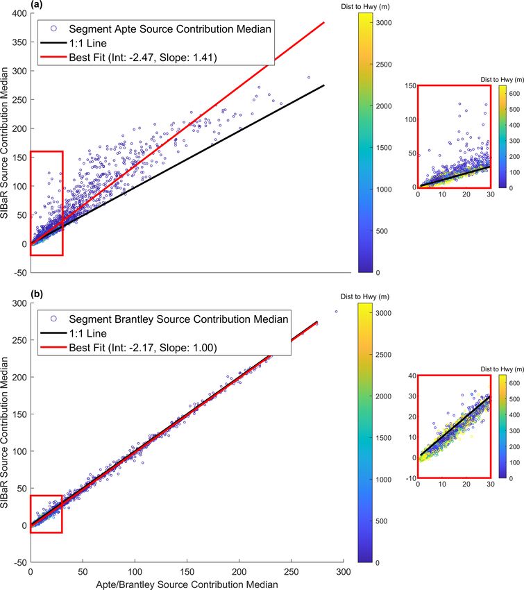
5812                                    B. Actkinson et al.: SIBaR: a new method for background quantification and removal

We define a variable δ recursively as                              in the percentage of correctly classified time series to range
                                                                between 80 %–100 %, dipping below 50 % only for the most
δt+1 (j ) = maxδt (i)aij p yt+1 |θj z                        (5)   stringent requirement (5 %). These results give us confidence
                                                                   in the partitioning step.
with the initialization
                                                                   2.3   Natural spline fit
δ1 (i) = πi p (y1 |θi z) .                                   (6)
                                                                   After HMMs have been fit to all time series data, natural
To retrieve the state sequence, we create a matrix ψ such that
                                                                   splines are fit to the background points by day. As in the work
ψ1 (i) = 0,     1≤i≤N                                        (7)   published by Brantley et al. (2019; “Brantley”), we select a
                                                                  natural spline basis with the degrees of freedom equal to the
ψt (j ) = argmax δt−1 (i)aij ,        1 ≤ j ≤ N, 2 ≤ t ≤ T . (8)   number of hours in the time series. However, we fit to the
                                                                   mean of our partitioned background time series, whereas in
We retrieve the state sequence by backtracking:
                                                                   Brantley the focus is on a 10th quantile regression. An exam-
qT = argmax [δT (i)] ,       1≤i≤N                           (9)   ple of this spline fit is given in Fig. 1.
                                                                     Because SIBaR’s partitioning step periodically generates
qt = ψt+1 (qt+1 ) ,      t = T − 1, T − 2, . . .1.          (10)
                                                                   background-assigned points that differ from one another for
This state sequence is then used to designate observations as      the same time series, we perform a test to evaluate its robust-
background or source. State-assigned points with the lower         ness. We run SIBaR 25 times and evaluate the pairwise root
median are designated background. An example of a decoded          mean square error (RMSE) between each set of generated
sequence is given in Fig. 1 for NOx (after retransformation).      background predictions for NOx as defined by
    HMM fits can be highly sensitive to time series outliers                  v
                                                                              uT
(Svensén and Bishop, 2005; Chatzis and Varvarigou, 2007;                      u (nta − ntb )2
                                                                              uP
Chatzis et al., 2009). Additionally, while computationally                    t t
                                                                   RMSE =                                                      (11)
cheap, the linearity assumption embedded in the time covari-                             T
ate could fail to capture more complex variations in back-
ground and produce flawed state categorizations. To capture        in which nta is the background realization at time t of signal
misclassification instances, we recast the step as an unsu-        a, ntb is the background realization at time t of signal b, and
pervised learning problem, design an empirical routine to          T is the total number of realizations in the time series.
evaluate the quality of created clusters, and incorporate it          The pairwise RMSE values for the first 12 runs are given in
into SIBaR. The routine, coined the fitted line classifier, fits   Table S3. We calculate an average RMSE of 0.05 ± 0.02 ppb
a line between averaged transition measurements and their          between each background signal and conclude that the fitting
corresponding transition times. The method then calculates         step is robust to small changes in background-assigned points
the percentage of points above the line that are classified as     in the partitioning step.
background and the percentage of points below the line that
                                                                   2.4   Evaluating the partitioning step: validation on an
are classified as source. If either percentage is greater than
                                                                         external dataset
or equal to 50 %, a predetermined percentage threshold, the
method deems the series incorrectly classified. If a series is     To test the validity of the partitioning step, we perform exter-
incorrectly classified, SIBaR breaks the series into two and       nal validation using a mobile monitoring dataset published
performs the background partitioning step on each half chunk       in Brantley et al. (2014). In that study, a van collecting mo-
separately. Sixteen example time series, labeled as classified     bile measurements of carbon monoxide (CO) systematically
correctly or incorrectly, are depicted in Figs. S1 and S2. After   looped a route in which it drove through a predefined back-
fitting HMMs to each separate chunk, SIBaR then uses the           ground location, on transects to a highway, and on the high-
fitted line classifier on each chunk, repeating the process if     way itself (Brantley et al., 2014). The measurements taken
any chunk’s partitioning is labeled misclassified. The process     in the prescribed background location were marked as back-
continues recursively until all created partitions are deemed      ground, and all other measurements were marked as non-
correctly classified. SIBaR then combines the state designa-       background. We run the partitioning step on these data to
tions from all created chunks into one and returns those state     determine how well SIBaR captures the measurements taken
designations as the corrected designations for the time series.    in the background location of the study.
    In running SIBaR on the campaign NOx measurements,
we note that the empirical classifier designates 96 % of the       2.5   Generating mapped fractional background
original time series to be correctly classified for a 50 %               contribution and source contribution maps
threshold. We run a sensitivity analysis on the percentage
threshold and show the results in Fig. S3. The figure illus-       We explore the spatial extent of our HMM-decoded catego-
trates that changing the percentage threshold causes changes       rizations from the partitioning step by creating mapped frac-

Atmos. Meas. Tech., 14, 5809–5821, 2021                                             https://doi.org/10.5194/amt-14-5809-2021
B. Actkinson et al.: SIBaR: a new method for background quantification and removal                                                         5813

Figure 1. Example time series of SIBaR background signal (blue) being fit to background designated points (black) created in the SIBaR
partitioning step. Points are colored red if designated as the source in the partitioning step and black if designated background. Data presented
in this time series were collected on 30 March 2018 starting at 10:00 Central Daylight Time (CDT).

tional background contribution maps. After aggregating time                using our method and the source contributions derived using
series observations (either CO2 or NOx , depending on the                  the other published methods.
pollutant analyzed) to road segment points created within our
road segment network, we sum the number of observations
designated as the background state and divide by the total                 3     Results – proof of concept
number of observations assigned to that road segment point.
                                                                           3.1    Validating the partitioning step on an external
We map the results and present them in Sect. 3.2.
                                                                                  dataset
   In Sect. 3.3, we derive source contributions (source sig-
nal = original signal – background signal) using our back-                 A comparison between SIBaR’s partitioning and the par-
ground method and map them. To put these source contri-                    titioning originally published by Brantley et al. (2014) is
butions in context with previously published work, we re-                  given in Fig. 2. Initially, the HMM fitting step is performed
peat the same process using background derived from a mov-                 and the resulting state sequence decoded. We run our clas-
ing 2 min 5th percentile baseline (Apte et al., 2017; “Apte”)              sifier on the initially decoded time series and find it to be
and the Brantley technique described previously in Sect. 2.2               misclassified, which is apparent from panel (a) of Fig. S4,
(Brantley et al., 2019). To derive our source contributions,               which shows the unsmoothed CO data before correction. The
we make predictions for the background for each time se-                   algorithm breaks the series into two chunks and refits the
ries realization collected using the derived background spline             HMM to each part separately, resulting in the state desig-
and then subtract those predictions from the original time se-             nations in panel (a) of Fig. 2. We then compute the per-
ries observations. We also derive source contributions using               centage of matching background/non-background designa-
the Apte and Brantley techniques. We create the maps using                 tions. The SIBaR partitioning step is able to match 83 %
the same methodology as Miller et al. (2020) and described                 of the originally published background/non-background des-
briefly here. Using our created road segment network, we                   ignations. The mismatches could be attributed to the tran-
take the mean of measurements collected as the GSV car                     sition between the background/non-background portions of
drives past a road segment point in our network, coined the                the route in the original study, which is observed in Fig. 2
drive pass mean. We take the median of these drive pass                    in the periods where background points show larger values
means and map the result. Because we consider drive pass                   than source points near periods of the transition (for example,
means taken within 4 h of one another to provide no new in-                the last blue spike at approximately 08:45 Eastern Daylight
formation about the air quality at that road segment, we take              Time, EDT). Mismatches also could be a result of the effects
the median of drive pass means occurring within that 4 h time              of traffic on measurements in the background designated por-
window to generate a 4 h median of drive pass means. Then,                 tion of the route. Finally, the mismatches could be attributed
we take the median of all 4 h medians of drive pass means                  to the inability of the SIBaR linearity assumption to capture
at that road segment to derive its map-reduced median. We                  finer scale temporal variations within the background (see
perform this procedure for the source contributions derived                Eqs. 2–4).

https://doi.org/10.5194/amt-14-5809-2021                                                       Atmos. Meas. Tech., 14, 5809–5821, 2021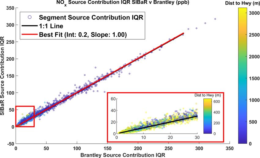
5814 B. Actkinson et al.: SIBaR: a new method for background quantification and removal
In running this test, we note that the method is sensitive 3.3 Comparison of source contribution maps using
to a smoothing time window if one is used. Figure S4 illus- different background removal techniques
trates uncorrected SIBaR-decoded states for three different
smoothing time windows on the same CO dataset and shows To put SIBaR predicted source contributions in context,
that the method produces different state categorizations de- we compare the source contribution maps generated using
pending on the window used, even making correction unnec- SIBaR to the ones generated by the Apte and Brantley tech-
essary in the 30 s instance. We hypothesize that smoothing niques. We zoom in on the Ship Channel domain for ease of
reduces the skewness of the data such that they better fit two comparison in Fig. 5. We refer the reader to Figs. S7–S15 to
switched lognormal Gaussian distributions. see maps for all other areas in the mobile monitoring cam-
paign for both NOx and CO2 . The average NOx background
3.2 Mapped fractional background state contributions predicted by the Apte, Brantley, and SIBaR techniques are
15.25, 11.58, and 13.02 ppb, respectively.
For the Houston mobile campaign, maps detailing the frac- Figure 5 shows that the source contributions derived using
tional contribution of the background state to the overall the Apte technique are lower on highways compared to the
mapped points are created for CO2 and NOx . Individual ob- source contributions derived using SIBaR and the Brantley
servations assigned to a road segment point have their de- techniques. Additionally, both the Brantley and SIBaR tech-
coded category designations assigned to the same point. The niques derive higher source contributions on road segments
number of observations assigned the background category with elevated NO and NO2 concentrations compared to the
are then divided by the total number of observations assigned Apte technique, as identified in Miller et al. (2020). We hy-
to the point to determine the fractional background state con- pothesize that this occurs due to the smaller time window uti-
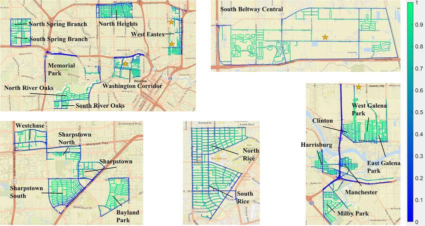
tribution. Figure 3 shows these census tract maps for NOx . lized in the Apte technique. The GSV vehicles would often
Figure S5 shows the maps for CO2 . It is important to note sit in traffic on highways for extended periods of time, mak-
that these maps represent the fraction of the measurements ing a 2 min time window unsuitable for describing source du-
that are categorized as background or source for the given rations during those time periods. While the 2 min assump-
pollutant at a given location. tion would be better suited for situations in which the car was
We note the following about the broad spatial patterns in exposed to source durations within that time interval (which
the mapped background state fraction presented in Fig. 3. occurred in the Apte study), it would not be for source dura-
First, background state designated points dominate residen- tions of a larger time interval, highlighting the challenges in
tial areas for both pollutants. This is encouraging, as it is ex- assuming a static time window for extensive mobile monitor-
pected that few point sources of these two pollutants would ing campaigns with varying source durations.
be found in residential neighborhoods except for those near We plot road segment median source contributions derived
industrial activity (Miller et al., 2020). Second, source state by Apte and Brantley algorithms against the road segment
designated points dominate highways and busy arterial roads, median concentrations derived by SIBaR and present the re-
which is expected given the large amounts of traffic on these sults for NOx in Fig. 6. Additionally, we plot lines of best fit
roads. Finally, we note the appearance of source-dominated derived using ordinary least squares (OLS) regression. Fig-
hotspots in front of point sources identified in our previous ure 6a illustrates that SIBaR derives higher source contri-
work (Miller et al., 2020) and denote their locations in Fig. 3. butions medians than the Apte technique, which is largely
This is encouraging given that we found these road segments driven by differences in highway road segment medians. The
to be elevated for NO and/or NO2 compared to their sur- slope determined using OLS regression suggests that, on av-
rounding neighborhood domain. erage, SIBaR median source contributions are ∼ 41 % higher
We take the background state fractions depicted in Fig. 3 than Apte median source contributions. Panel (b) of Fig. 6
and bin them by distance to the highway. The results are pre- comparing Brantley and SIBaR road segment medians in-
sented in Fig. 4. We do the same for CO2 and present the dicates much closer agreement between the two techniques,
results in Figs. S5–S6. The exponential behavior exhibited with SIBaR estimating source contribution medians at an av-
in Fig. 4 mirrors published exponential decays in roadside erage offset of 2 ppb lower than Brantley source contribu-
source pollutant concentrations (Apte et al., 2017; Karner et tion medians. Data for CO2 source contribution medians are
al., 2010), while the sizable interquartile ranges within each shown in Figs. S16 and S17.
bin highlight the complexity and variability of source road- While the road segment median source contributions be-
side gradients, which depend on emission rates, meteorology, tween the Brantley and SIBaR techniques exhibit strong
geography, and other factors (Baldwin et al., 2015; Patton et agreement, we note that source contributions evaluated on
al., 2014). a more granular level exhibit some disagreement. Figure 7
displays the inter quartile ranges (IQRs) for source contri-
butions assigned to each road segment plotted against each
other for the SIBaR and Brantley techniques, again colored
by distance to the closest highway. We display additional 1 : 1
Atmos. Meas. Tech., 14, 5809–5821, 2021 https://doi.org/10.5194/amt-14-5809-2021B. Actkinson et al.: SIBaR: a new method for background quantification and removal 5815 Figure 2. Comparison between SIBaR-predicted background and source states and originally published designations from Brantley et al. (2014) for log-transformed CO. Background designated points are in blue and source designated points in red. (a) SIBaR-decoded states for the mobile CO measurements. (b) Designations originally published by the authors of the study. Figure 3. Fraction of points aggregated to the road segment network designated as background in SIBaR-decoded states for NOx . Maps were generated following the methods outlined in Sect. 2.5. Points are mapped on a scale of 0 to 1; 1 implies all points aggregated to that road segment were designated as background and 0 implies all points were designated as non-background. Details of the census tracts are provided in Table S1. Gold stars indicate locations of elevated NO and/or NO2 medians next to known industrial facilities published in Miller et al. (2020). Basemap generated by MATLAB geobasemap “streets” and is hosted by ESRI (Sources: Esri, DeLorme, HERE, USGS, Intermap, iPC, NRCAN, Esri Japan, METI, Esri China (Hong Kong), Esri (Thailand), MapmyIndia, Tomtom). https://doi.org/10.5194/amt-14-5809-2021 Atmos. Meas. Tech., 14, 5809–5821, 2021
5816                                  B. Actkinson et al.: SIBaR: a new method for background quantification and removal

Figure 4. Boxplots of mapped background NOx fractions, presented in Fig. 3, binned by distance from the highway. The red line represents
the median, the top and bottom edges represent the 75th and 25th percentiles, respectively, and the whiskers extend to the most extreme data
points not considered outliers.

Figure 5. Comparison of source contributions derived using different techniques in the Ship Channel domain. Source contributions were
aggregated according to the methods described in Sect. 2.4. (a) Source contributions derived using the Apte technique. (b) Source contribu-
tions derived using the Brantley technique. (c) Source contributions derived using the SIBaR technique. Basemap generated by MATLAB
geobasemap “streets” and is hosted by ESRI (Sources: Esri, DeLorme, HERE, USGS, Intermap, iPC, NRCAN, Esri Japan, METI, Esri China
(Hong Kong), Esri (Thailand), MapmyIndia, Tomtom).

plots of the IQR for different techniques and pollutants (NOx           the two techniques. While SIBaR predicts lower source con-
and CO2 ) in the Supplement (Figs. S18–S20). There are no-              tributions compared to the Brantley technique on average,
ticeable deviations from the 1 : 1 line in IQR between SIBaR            there are noticeable discrepancies captured in the tails of the
and the Brantley technique for both NOx and CO2 , suggest-              distribution.
ing that the two techniques disagree with one another on indi-             To provide further context for these results, we present two
vidual source contribution drive pass means. Figure S21 dis-            examples of daily time series of each background technique’s
plays a histogram of differences in drive pass means between            predictions in Fig. 8. It is apparent that the Apte technique

Atmos. Meas. Tech., 14, 5809–5821, 2021                                                    https://doi.org/10.5194/amt-14-5809-2021
B. Actkinson et al.: SIBaR: a new method for background quantification and removal                                                        5817

Figure 6. Scatterplots of road segment median source contributions predicted by two different techniques against their corresponding SIBaR
median source contributions for NOx . The line of best fit is derived using OLS regression and is depicted in red. The 1 : 1 line is depicted in
black. Points are colored by their distance to the closest highway. (a) SIBaR source contribution medians plotted against Apte source con-
tribution medians. (b) SIBaR source contribution medians plotted against Brantley source contribution medians. The plots in red rectangles
designate a blown-up portion near the origin.

overfits to the data in both cases. The top panel shows an                dictions that are captured in the left tail of the histogram in
example of SIBaR’s predictions offering an advantage over                 Fig. S21. Both panels illustrate why the medians of Brantley
Brantley’s; since SIBaR is fit to a subset of the data, it avoids         and SIBaR agree so well with one another, yet display IQRs
overfitting in the early morning hours of the time series that            that deviate from their 1 : 1 line. Both signals exhibit strong
the Brantley time series incorporates. Figure 8a illustrates              agreement with one another but can capture different source
why the cases in the right tail of the histogram in S21 exist.            influences periodically because of the assumptions inherent
In contrast, the bottom panel showcases the potential faults in           in each technique. It is also evident that the appropriate back-
using SIBaR predictions; since there are no background des-               ground fit would need to be investigated on a case-by-case
ignated points at the beginning of this time series example,              basis, as one should avoid using the SIBaR technique in in-
the spline fit wildly extrapolates, resulting in unrealistic pre-         stances where extrapolation could occur.

https://doi.org/10.5194/amt-14-5809-2021                                                      Atmos. Meas. Tech., 14, 5809–5821, 2021
5818                                   B. Actkinson et al.: SIBaR: a new method for background quantification and removal

Figure 7. 1 : 1 scatterplot of the interquartile range (IQR) of predicted NOx source contributions at individual road segments for the SIBaR
and Brantley techniques. The line of best fit is derived using OLS regression and is depicted in red. The 1 : 1 line is depicted in black. The
inset, outlined by the red rectangle, shows the IQR at lower values of the Brantley source contribution IQR. Deviations from the 1 : 1 line
suggest that SIBaR captures source influences the Brantley method fails to detect, despite predicting lower source contributions on average
and the excellent agreement in median source contribution.

4   Concluding remarks                                                   predictions for transformed (Fig. 9a) and non-transformed
                                                                         (Fig. 9b) NOx data. The transformation in this instance re-
We illustrate that SIBaR provides a defensible mechanism                 sults in portions of the measurements in the early morning
to quantify and remove background from air pollution mon-                period being classified as background, whereas none are des-
itoring data time series. The method’s partitioning step                 ignated as background in the non-transformed case. While
is able to match 83 % of a study’s previously published                  we think data are more appropriately described in the log-
background/non-background designations. Mapped distribu-                 normal regime (Seinfeld and Pandis, 2016), careful consid-
tions of the partitioning step’s decoded states show high lev-           eration of transformation is necessary. Additionally, as dis-
els of background state assignment in residential areas, with            cussed in Sect. 3.1 and exhibited in Fig. S4, applying a
notable exceptions in hotspots published in a previous study.            smoothing time window can also affect the state categoriza-
Finally, we show the impact using SIBaR can have on deriv-               tions.
ing source contributions in comparing it to the background                  While the linearity assumption in the time covariate is
signals predicted by other techniques. Most notably, SIBaR               computationally cheap and easy to implement, it is limited.
does not rely on a static time window assumption to deter-               It is unrealistic to expect background air pollution to exhibit
mine source impacts, and instead relies on fitting to a subset           linear behavior, especially as the time series duration extends
of the data generated with a time series regime change mod-              (Luke et al., 2010). While the linearity assumption seems to
eling technique. Setting a static time window can have signif-           be acceptable for time series of several hours of data, prob-
icant impact on the derived source contributions, as exhibited           lems with that assumption arose in this work and will most
by the discrepancies between the Apte and SIBaR methods                  likely arise on time series of data by day or when time series
shown in Sect. 3.3. While the SIBaR and Brantley techniques              are impacted by abrupt meteorological changes. Future work
produce similar source contribution medians to one another               should incorporate assumptions of non-linear behavior into
in the context of this campaign’s measurements, both capture             the analysis. Several studies have been published showing
different source influences based on the assumptions inherent            the applicability of HMMs to covariates expressed as splines
in each respective technique.                                            (Langrock et al., 2015, 2018). However, trade-offs between
   Despite SIBaR’s rigor and advancements relative to pre-               computational time and precision would need to be consid-
viously published methods, our approach needs careful con-               ered. In its current version, SIBaR takes ∼ 6.5 h to model
sideration and improvement. The method is sensitive to how               background for millions of data points (performing the por-
data in the time series are distributed, and transforming the            tioning step, evaluating and/or correcting the fit, and fitting
measurements can provide different results. For example,                 the spline for all time series). The Brantley technique, in con-
Fig. 9 exhibits a side-by-side comparison of SIBaR state                 trast, takes several minutes.

Atmos. Meas. Tech., 14, 5809–5821, 2021                                                     https://doi.org/10.5194/amt-14-5809-2021
B. Actkinson et al.: SIBaR: a new method for background quantification and removal 5819 Figure 8. Time series plots depicting the original mobile campaign measurements, colored by their SIBaR-decoded states (background and source), along with the background signals generated by the SIBaR, Brantley, and Apte techniques. (a) NOx time series of mobile measurements taken on 3 October 2017, which displays the Apte and Brantley signals overfitting to data decoded as source by the SIBaR partitioning step. (b) NOx time series of mobile measurements taken on 30 November 2017, which shows wildly extrapolated SIBaR predictions at the beginning of the time series due to the lack of background-decoded states. Figure 9. Comparison of SIBaR state designations for (a) log-transformed versus (b) non-transformed NOx data on 30 October 2017 (local time, i.e., Central Daylight Time, CDT) in the Houston mobile monitoring campaign. Transformation can affect state assignments, which in this case results in 38 % of the observations having a different categorization upon transformation. Despite these shortcomings, SIBaR holds promise as a partitioning step captures transient behavior between back- framework to quantify and remove background from air pol- ground and non-background quite well, as the diagnostic re- lution monitoring time series. In its current state, it is inferior sults of Sect. 3.1 and the maps in Sect. 3.2 indicate. In addi- to the Brantley technique with regards to computation time. tion to addressing other issues highlighted here, future work However, these problems with SIBaR are computational ones should focus on methods to reduce its computational time to rather than problems with its underlying theory. The SIBaR make its use more straightforward. https://doi.org/10.5194/amt-14-5809-2021 Atmos. Meas. Tech., 14, 5809–5821, 2021
5820                                   B. Actkinson et al.: SIBaR: a new method for background quantification and removal

Code and data availability. Both the code and data are available on     Baldwin, N., Gilani, O., Raja, S., Batterman, S., Ganguly,
request. Additionally, time series comparisons for all 312 time se-       R., Hopke, P., Berrocal, V., Robins, T., and Hoogterp,
ries taken in the campaign, as well as a demo of the SIBaR partition-     S.: Factors affecting pollutant concentrations in the
ing step, are available at https://doi.org/10.5281/zenodo.5022590         near-road environment, Atmos. Environ., 115, 223–235,
(Actkinson et al., 2021). Data are also free to download from Ope-        https://doi.org/10.1016/j.atmosenv.2015.05.024, 2015.
nAQ (https://openaq.org/#/project/28974, Environmental Defense          Brantley, H. L., Hagler, G. S. W., Kimbrough, E. S., Williams, R.
Fund, 2021).                                                              W., Mukerjee, S., and Neas, L. M.: Mobile air monitoring data-
                                                                          processing strategies and effects on spatial air pollution trends,
                                                                          Atmos. Meas. Tech., 7, 2169–2183, https://doi.org/10.5194/amt-
Supplement. The supplement related to this article is available on-       7-2169-2014, 2014.
line at: https://doi.org/10.5194/amt-14-5809-2021-supplement.           Brantley, H. L., Hagler, G. S. W., Herndon, S. C., Massoli, P.,
                                                                          Bergin, M. H., and Russell, A. G.: Characterization of Spa-
                                                                          tial Air Pollution Patterns Near a Large Railyard Area in At-
Author contributions. BA developed, wrote, and tested the method          lanta, Georgia, Int. J. Environ. Res. Public. Health, 16, 535,
in R (R: The R Project for Statistical Computing, 2021) with crit-        https://doi.org/10.3390/ijerph16040535, 2019.
ical input and scientific guidance from RJG and KE. RJG super-          Bukowiecki, N., Dommen, J., Prévôt, A. S. H., Richter, R., Wein-
vised the project and provided feedback on the significance of the        gartner, E., and Baltensperger, U.: A mobile pollutant measure-
method’s results. BA wrote the manuscript. All authors contributed        ment laboratory – measuring gas phase and aerosol ambient
to the editing and review of the manuscript.                              concentrations with high spatial and temporal resolution, At-
                                                                          mos. Environ., 36, 5569–5579, https://doi.org/10.1016/S1352-
                                                                          2310(02)00694-5, 2002.
                                                                        Caplin, A., Ghandehari, M., Lim, C., Glimcher, P., and
Competing interests. The authors declare that they have no conflict
                                                                          Thurston, G.: Advancing environmental exposure assess-
of interest.
                                                                          ment science to benefit society, Nat. Commun., 10, 1–11,
                                                                          https://doi.org/10.1038/s41467-019-09155-4, 2019.
                                                                        Chambliss, S. E., Preble, C. V., Caubel, J. J., Cados, T., Messier, K.
Disclaimer. Publisher’s note: Copernicus Publications remains             P., Alvarez, R. A., LaFranchi, B., Lunden, M., Marshall, J. D.,
neutral with regard to jurisdictional claims in published maps and        Szpiro, A. A., Kirchstetter, T. W., and Apte, J. S.: Comparison
institutional affiliations.                                               of Mobile and Fixed-Site Black Carbon Measurements for High-
                                                                          Resolution Urban Pollution Mapping, Environ. Sci. Technol., 54,
                                                                          7848–7857, https://doi.org/10.1021/acs.est.0c01409, 2020.
Acknowledgements. We thank Halley Brantley for the provision of         Chatzis, S. and Varvarigou, T.: A Robust to Outliers Hid-
data and comments concerning results in Sect. 3.1 of the paper. We        den Markov Model with Application in Text-Dependent
also appreciate support from the Environmental Defense Fund for           Speaker Identification, in: 2007 IEEE International Con-
the collection and provision of mobile data.                              ference on Signal Processing and Communications, 24–
                                                                          27 November 2007, Dubai, United Arab Emirates, 804–807,
                                                                          https://doi.org/10.1109/ICSPC.2007.4728441, 2007.
Financial support. This research has been supported by the              Chatzis, S. P., Kosmopoulos, D. I., and Varvarigou, T. A.: Ro-
National Institute of Environmental Health Sciences (grant                bust Sequential Data Modeling Using an Outlier Tolerant Hid-
no. R01ES028819-01).                                                      den Markov Model, IEEE Trans. Pattern Anal. Mach. Intell., 31,
                                                                          1657–1669, https://doi.org/10.1109/TPAMI.2008.215, 2009.
                                                                        Dempster, A. P., Laird, N. M., and Rubin, D. B.: Maximum Like-
Review statement. This paper was edited by Glenn Wolfe and re-            lihood from Incomplete Data Via the EM Algorithm, J. R. Stat.
viewed by two anonymous referees.                                         Soc. Ser. B Methodol., 39, 1–22, https://doi.org/10.1111/j.2517-
                                                                          6161.1977.tb01600.x, 1977.
                                                                        Environmental Defense Fund: Google Earth Outreach, Rice Univer-
                                                                          sity, and Sonoma Technology: Houston Mobile, OpenAQ [data
References                                                                set], available at: https://openaq.org/#/project/28974, last access:
                                                                          18 August 2021.
Actkinson, B., Ensor, K., and Griffin, R. J.: Time Series Com-          Forney, G. D.: The viterbi algorithm, Proc. IEEE, 61, 268–278,
  parisons, Model Code, and a Demo Dataset for SIBaR: A                   https://doi.org/10.1109/PROC.1973.9030, 1973.
  New Method for Background Quantification and Removal                  Gómez-Losada, Á., Pires, J. C. M., and Pino-Mejías, R.:
  from Mobile Air Pollution Measurements, Zenodo [data set],              Characterization of background air pollution exposure
  https://doi.org/10.5281/zenodo.5022590, 2021.                           in urban environments using a metric based on Hid-
Apte, J. S., Messier, K. P., Gani, S., Brauer, M., Kirchstet-             den Markov Models, Atmos. Environ., 127, 255–261,
  ter, T. W., Lunden, M. M., Marshall, J. D., Portier, C. J.,             https://doi.org/10.1016/j.atmosenv.2015.12.046, 2016.
  Vermeulen, R. C. H., and Hamburg, S. P.: High-Resolution              Gómez-Losada, Á., Pires, J. C. M., and Pino-Mejías, R.: Modelling
  Air Pollution Mapping with Google Street View Cars: Ex-                 background air pollution exposure in urban environments: Im-
  ploiting Big Data, Environ. Sci. Technol., 51, 6999–7008,
  https://doi.org/10.1021/acs.est.7b00891, 2017.

Atmos. Meas. Tech., 14, 5809–5821, 2021                                                    https://doi.org/10.5194/amt-14-5809-2021
B. Actkinson et al.: SIBaR: a new method for background quantification and removal 5821 plications for epidemiological research, Environ. Model. Softw., Miller, D. J., Actkinson, B., Padilla, L., Griffin, R. J., Moore, 106, 13–21, https://doi.org/10.1016/j.envsoft.2018.02.011, 2018. K., Lewis, P. G. T., Gardner-Frolick, R., Craft, E., Portier, C. Gómez-Losada, Á., Santos, F. M., Gibert, K., and Pires, J. C. M.: A J., Hamburg, S. P., and Alvarez, R. A.: Characterizing Ele- data science approach for spatiotemporal modelling of low and vated Urban Air Pollutant Spatial Patterns with Mobile Monitor- resident air pollution in Madrid (Spain): Implications for epi- ing in Houston, Texas, Environ. Sci. Technol., 54, 2133–2142, demiological studies, Comput. Environ. Urban Syst., 75, 1–11, https://doi.org/10.1021/acs.est.9b05523, 2020. https://doi.org/10.1016/j.compenvurbsys.2018.12.005, 2019. Patton, A. P., Perkins, J., Zamore, W., Levy, J. I., Brugge, Hankey, S. and Marshall, J. D.: Land Use Regression Mod- D., and Durant, J. L.: Spatial and temporal differences els of On-Road Particulate Air Pollution (Particle Num- in traffic-related air pollution in three urban neighborhoods ber, Black Carbon, PM2.5 , Particle Size) Using Mo- near an interstate highway, Atmos. Environ., 99, 309–321, bile Monitoring, Environ. Sci. Technol., 49, 9194–9202, https://doi.org/10.1016/j.atmosenv.2014.09.072, 2014. https://doi.org/10.1021/acs.est.5b01209, 2015. R: The R Project for Statistical Computing, available at: https: Hankey, S., Sforza, P., and Pierson, M.: Using Mobile Monitoring //www.r-project.org/, last access: 22 June 2021. to Develop Hourly Empirical Models of Particulate Air Pollution Robinson, E. S., Gu, P., Ye, Q., Li, H. Z., Shah, R. U., in a Rural Appalachian Community, Environ. Sci. Technol., 53, Apte, J. S., Robinson, A. L., and Presto, A. A.: Restau- 4305–4315, https://doi.org/10.1021/acs.est.8b05249, 2019. rant Impacts on Outdoor Air Quality: Elevated Organic Hudda, N., Gould, T., Hartin, K., Larson, T. V., and Fruin, S. A.: Aerosol Mass from Restaurant Cooking with Neighborhood- Emissions from an International Airport Increase Particle Num- Scale Plume Extents, Environ. Sci. Technol., 52, 9285–9294, ber Concentrations 4-fold at 10 km Downwind, Environ. Sci. https://doi.org/10.1021/acs.est.8b02654, 2018. Technol., 48, 6628–6635, https://doi.org/10.1021/es5001566, Seinfeld, J. H. and Pandis, S. N.: Atmospheric Chemistry and 2014. Physics: From Air Pollution to Climate Change, John Wiley & Karner, A. A., Eisinger, D. S., and Niemeier, D. A.: Near- Sons, Hoboken, New Jersey, USA, 1146 pp., 2016. Roadway Air Quality: Synthesizing the Findings from Shairsingh, K. K., Jeong, C.-H., Wang, J. M., and Evans, Real-World Data, Environ. Sci. Technol., 44, 5334–5344, G. J.: Characterizing the spatial variability of local and https://doi.org/10.1021/es100008x, 2010. background concentration signals for air pollution at Langrock, R., Kneib, T., Sohn, A., and DeRuiter, S. L.: Nonpara- the neighbourhood scale, Atmos. Environ., 183, 57–68, metric inference in hidden Markov models using P-splines, Bio- https://doi.org/10.1016/j.atmosenv.2018.04.010, 2018. metrics, 71, 520–528, https://doi.org/10.1111/biom.12282, 2015. Svensén, M. and Bishop, C. M.: Robust Bayesian Langrock, R., Adam, T., Leos-Barajas, V., Mews, S., Miller, D. L., mixture modelling, Neurocomputing, 64, 235–252, and Papastamatiou, Y. P.: Spline-based nonparametric inference https://doi.org/10.1016/j.neucom.2004.11.018, 2005. in general state-switching models, Stat. Neerlandica, 72, 179– Tessum, M. W., Larson, T., Gould, T. R., Simpson, C. D., Yost, 200, https://doi.org/10.1111/stan.12133, 2018. M. G., and Vedal, S.: Mobile and Fixed-Site Measurements Larson, T., Gould, T., Riley, E. A., Austin, E., Fintzi, J., Sheppard, To Identify Spatial Distributions of Traffic-Related Pollution L., Yost, M., and Simpson, C.: Ambient air quality measure- Sources in Los Angeles, Environ. Sci. Technol., 52, 2844–2853, ments from a continuously moving mobile platform: Estimation https://doi.org/10.1021/acs.est.7b04889, 2018. of area-wide, fuel-based, mobile source emission factors using TIGER/Line Shapefile: Harris County, TX, All absolute principal component scores, Atmos. Environ., 152, 201– Roads County-based Shapefile, available at: 211, https://doi.org/10.1016/j.atmosenv.2016.12.037, 2017. https://catalog.data.gov/dataset/tiger-line-shapefile-2018- Li, H. Z., Gu, P., Ye, Q., Zimmerman, N., Robinson, E. county-harris-county-tx-all-roads-county-based-shapefile (last S., Subramanian, R., Apte, J. S., Robinson, A. L., and access: 19 October 2020), 2018. Presto, A. A.: Spatially dense air pollutant sampling: Impli- Van den Bossche, J., Peters, J., Verwaeren, J., Botteldooren, cations of spatial variability on the representativeness of sta- D., Theunis, J., and De Baets, B.: Mobile monitoring tionary air pollutant monitors, Atmos. Environ., 2, 100012, for mapping spatial variation in urban air quality: De- https://doi.org/10.1016/j.aeaoa.2019.100012, 2019. velopment and validation of a methodology based on Luke, W. T., Kelley, P., Lefer, B. L., Flynn, J., Rappenglück, B., an extensive dataset, Atmos. Environ., 105, 148–161, Leuchner, M., Dibb, J. E., Ziemba, L. D., Anderson, C. H., and https://doi.org/10.1016/j.atmosenv.2015.01.017, 2015. Buhr, M.: Measurements of primary trace gases and NOY com- Visser, I. and Speekenbrink, M.: depmixS4: An R Pack- position in Houston, Texas, Atmos. Environ., 44, 4068–4080, age for Hidden Markov Models, J. Stat. Softw., 36, 1–21, https://doi.org/10.1016/j.atmosenv.2009.08.014, 2010. https://doi.org/10.18637/jss.v036.i07, 2010. Messier, K. P., Chambliss, S. E., Gani, S., Alvarez, R., Brauer, M., Zhang, X., Chen, X., and Zhang, X.: The impact of exposure to air Choi, J. J., Hamburg, S. P., Kerckhoffs, J., LaFranchi, B., Lun- pollution on cognitive performance, Proc. Natl. Acad. Sci. USA, den, M. M., Marshall, J. D., Portier, C. J., Roy, A., Szpiro, A. 115, 9193–9197, https://doi.org/10.1073/pnas.1809474115, A., Vermeulen, R. C. H., and Apte, J. S.: Mapping Air Pollution 2018. with Google Street View Cars: Efficient Approaches with Mobile Monitoring and Land Use Regression, Environ. Sci. Technol., 52, 12563–12572, https://doi.org/10.1021/acs.est.8b03395, 2018. https://doi.org/10.5194/amt-14-5809-2021 Atmos. Meas. Tech., 14, 5809–5821, 2021
You can also read