Size and long-term growth trends of Endangered fish-eating killer whales
←
→
Page content transcription
If your browser does not render page correctly, please read the page content below
Vol. 13: 173–180, 2011                    ENDANGERED SPECIES RESEARCH
                                                                                                               Published online March 9
      doi: 10.3354/esr00330                        Endang Species Res

                                                                                                                      OPEN
                                                                                                                      ACCESS

  Size and long-term growth trends of Endangered
              fish-eating killer whales
     Holly Fearnbach1,*, John W. Durban2, 3, Dave K. Ellifrit2, Ken C. Balcomb III2
         1
         School of Biology, University of Aberdeen, Lighthouse Field Station, Cromarty, Ross-shire IV11 8YJ, UK
                          2
                           Center for Whale Research, Friday Harbor, Washington 98250, USA
          3
           Protected Resources Division, Southwest Fisheries Science Center, National Marine Fisheries Service,
      National Oceanic and Atmospheric Administration, 8604 La Jolla Shores Drive, La Jolla, California 92037, USA

       ABSTRACT: The Endangered southern resident population of killer whales Orcinus orca has been
       shown to be food-limited, and the availability of their primary prey, Chinook salmon Oncorhynchus
       tshawytscha, has been identified as a key covariate for the whales’ individual survival and reproduc-
       tion. We collected aerial photogrammetry data on individual whale size, which will help to better
       inform energetic calculations of food requirements, and we compared size-at-age data to make infer-
       ences about long-term growth trends. A helicopter was used to conduct 10 flights in September 2008,
       resulting in 2803 images from which useable measurements were possible for 66 individually identi-
       fiable whales, representing more than three-quarters of the population. Estimated whale lengths
       ranged from 2.7 m for a neonate whale in its first year of life, to a maximum of 7.2 m for a 31 yr old
       adult male. Adult males reached an average (asymptotic) size estimate (± SE) of 6.9 ± 0.2 m, with
       growth slowing notably after the age of 18 yr; this was significantly larger than the asymptotic size of
       6.0 ± 0.1 m for females, which was reached after the earlier age of 15 yr. Notably, there was no over-
       lap between the ranges of estimated sizes of adult males (6.5 to 7.2 m) and females (5.5 to 6.4 m). On
       average, older adults (> 30 yr) were 0.3 m (n = 14, p = 0.03) and 0.3 m (n = 5, p = 0.23) longer than the
       younger whales of adult age, for females and males, respectively; we hypothesize that a long-term
       reduction in food availability may have reduced early growth rates and subsequent adult size in
       recent decades.

       KEY WORDS: Killer whale · Photogrammetry · Size · Growth · Salmon
                              Resale or republication not permitted without written consent of the publisher

                    INTRODUCTION                                        adult size is influenced by environmental factors during
                                                                        early growth (Metcalfe & Monaghan 2001, Catchpole et
   Data on individual size of organisms can be used to ad-              al. 2004), and therefore information on size and size
dress fundamental questions with respect to conserva-                   trends can be used to infer responses to environmental
tion management of Endangered populations. These                        variability, such as the effects of nutritional stress due to
fundamental questions include identification of taxo-                   limited food availability (Choquenot 1991, Catchpole et
nomic status (Perryman & Lynn 1993, Perryman & West-                    al. 2000, Trites & Donnelly 2003).
lake 1998, Pitman et al. 2007), assessment of health                      Free-ranging cetaceans at sea represent a challenge
(Choquenot 1991, Landete-Castillejos et al. 2002, Perry-                for collecting morphometric data, although live-capture
man & Lynn 2002), estimation of energetic requirements                  operations have been possible for some smaller species
(Williams et al. 2004, Noren 2011), and identification of               (e.g. Read et al. 1993). Photogrammetric approaches
key life-history and demographic patterns (Choquenot                    implemented from boat-based platforms have provided
1991, Koski et al. 1992, Perryman & Lynn 1993, Read et                  a simple alternative for measuring body features ex-
al. 1993, Lee & Moss 1995, Flamm et al. 2000, Shrader et                posed above the surface (Durban & Parsons 2006, Ja-
al. 2006, Breuer et al. 2007). Notably, an individual’s                 quet 2006, Webster et. al. 2010), but precise estimates

*Email: holly.fearnbach@noaa.gov                                        © Inter-Research 2011 · www.int-res.com
174 Endang Species Res 13: 173–180, 2011 of full body size typically require an aerial platform to physically immature animals (Olesiuk et al. 1990), and obtain through-water images from directly above a age data are not available, constraining a detailed as- whale (Koski et al. 1992, Perryman & Lynn 1993, 2002, sessment of the full size-at-age profile and preventing Perryman & Westlake 1998). Helicopter platforms have use of these data for examining size trends. A key fea- proven to be extremely well suited to providing precise ture of our approach was the use of an established long- photogrammetric measurements of cetaceans (e.g. Pit- term photo-identification catalog of individuals (Ford et man et al. 2007), due largely to the ability of helicopters al. 2000) to match aerial photographs and measure- to hover at a fixed (and known) altitude and make rela- ments to individual whales of known sex and age (Ole- tively subtle adjustments in location to remain directly siuk et al. 1990, Ford et al. 2000). Aerial photographic overhead of target animals. Although helicopters have surveys were directed in real-time by boat-based been deployed for this purpose from pelagic research photo-identification surveys to maximize the coverage ships (Perryman & Lynn 1993), they offer particular of different individuals and age/sex classes within the utility for aerial photogrammetry of accessible coastal population. populations that can be surveyed during short (fuel- restricted) helicopter flights with minimal open-water flying. MATERIALS AND METHODS The Endangered southern resident population of killer whales Orcinus orca is one of the most accessi- Field methods. We used a Robinson R44 Clipper ble populations of cetaceans. This distinct population helicopter to survey for whales from an airport at Fri- comprises 25 yr of experience in recog- the USA. nizing individual southern resident killer whales at Long-term prey-habit studies of southern resident sea. The helicopter then hovered to hold position over killer whales have shown distinct prey specialization each target whale until the photographer (H.F.) had on Chinook salmon Oncorhynchus tshawytscha during captured suitable images of the whale. the summer months (Ford & Ellis 2006), and recent The photographer was positioned in the passenger analysis of long-term demographic data has shown this seat behind the pilot so that both could obtain a similar whale population to be food-limited, with declines in view from the same side of the helicopter, which facili- survival (Ford et al. 2009), fecundity (Ward et al. 2009), tated positioning directly overhead of the whale. and social cohesion (Parsons et al. 2009) during years Wearing a seat harness, the photographer then leaned with low Chinook salmon availability. The aims of the out of the open passenger door to shoot photographs present study were (1) to collect aerial photogramme- vertically down on the target whale. A bubble-level try data on individual size, which will help to better was attached to the back of a hand-held digital SLR inform energetic calculations of food requirements for camera (Nikon D300), to ensure that the camera was this population (Noren 2011), and (2) to compare size- orientated vertically, while the photographer used con- at-age data to make inferences about long-term tinuous shooting mode to capture as many images as growth trends. possible of the surfacing whale. Photographs were Existing size data are available for > 30 individuals taken when the whale was at the water surface and from this population that were captured in a live- parallel to the water surface. High-quality JPEG capture fishery for exhibition in aquaria, conducted in images were shot at a resolution of 4288 × 2848 pixels the 1960s and early 1970s (Bigg & Wolman 1975, Ole- (13.1 megapixel resolution) in preference to raw siuk et al. 1990). However, this fishery selected for images in order to maximize the number of frames per
Fearnbach et al.: Size and growth of killer whales 175
second (to ~6 frames s–1). This ensured that the most ing the identification catalog, and then to select the
elongated position of the whale was captured on each best image(s) from each surfacing sequence of an
surfacing. A fixed focal length 180 mm f2.8 AF Nikkor identified whale. To ensure high quality, only images
lens was used either with or without a 1.4× Kenko Pro that were deemed to be vertical and with the whale in
extender, to achieve a realized focal length of either straight orientation (i.e. body axis of the whale was
378 or 270 mm (after accounting for the focal length not tilted) were selected, and the most elongated
factor of 1.5 inherent in the digital image sensor of the image(s) of each whale was then chosen from the fil-
camera). tered set from each surfacing. The freely available
The altitude was recorded at 1 s intervals throughout software ImageJ (http://rsbweb.nih.gov/ij/) was used
each flight using an onboard Garmin GPSMap 396 aer- to measure the distance (in pixels) between the tip of
ial GPS unit. This WAAS-enabled (WAAS: Wide Area upper jaw to the notch in the flukes (e.g. Pitman et al.
Augmentation System) differential GPS continuously 2007). All measurements in pixels were first con-
received parallel signals from 12 satellites, and also verted to a true measurement based on the actual
calibration signals from shore stations, to compute and width of the digital sensor (0.036 m) and the dimen-
update the position with advertised error of < 3 m sions of this sensor width in pixels (4288). These mea-
(www8.garmin.com/aboutGPS/waas.html). The GPS sured distances were then converted to true lengths
and camera time were synchronized so that each based on the scale of each image, which was calcu-
image could be linked to a specific altitude using a lated from the known altitude and realized lens focal
relational database. To ensure that these 2 time stamps length (scale = altitude/focal length). Images and
were precisely matched, a Blue2Can Bluetooth re- associated data on individual identification, individual
ceiver on the camera received wireless time signals age, focal length, and size measurements were
from a second GPS unit (Holux M241), and this time imported into a Microsoft Access relational database,
was directly embedded into the metadata associated where they were linked to the GPS data on altitude
with each image. This ensured that both the altitude- based on the time matches.
linked aerial GPS time and the camera time were To test the variability in our technique, we used aer-
derived from GPS signals, rather than relying on the ial photographs to estimate the size of boats of known
pre-set camera clock that had to be manually updated. length. To be consistent with the whale measurements,
Photographic processing. Prior to measuring, every we used 2 research vessels, which were photographed
photograph was examined by D.K.E. to match the in the same locations and at the same time as photo-
image to an individual whale. The digital photographs graphic encounters with whales. Conveniently, these
were displayed on a 22-inch (56 cm) high-resolution boats were the same approximate size as whales from
flat panel monitor and were viewed
through ACDSee photo manager
(www.acdsee.com/). Photographs were
linked to known individuals (of known
age and sex class) by matching saddle-
patch pigmentation patterns (Fig. 1)
of individual whales to the long-term
(33 yr) identification catalog (Ford et al.
2000, K. C. Balcomb unpubl. data). Pho-
tographic matches to the catalog were
validated, where possible, by examin-
ing identification photographs obtained
during the coordinated boat-based
operations, and also using boat-based
records of group composition and spac-
ing at times coincidental to the aerial
photographs.
Photographs of identified whales
were then re-examined by H.F. for
measurement purposes, again using a
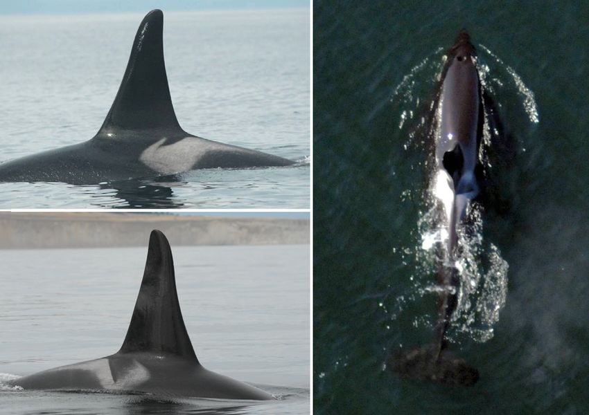
22-inch (56 cm) high-resolution moni- Fig. 1. Left-side (upper left panel) and right-side (lower left panel) identification
photographs obtained from boat platforms of Whale L78, a male first seen as
tor. ACDSee photo manager was first a young-of-the-year in 1989, displaying the distinctive saddle-patch pigmenta-
used to perform a second check of the tion of southern resident killer whales Orcinus orca which is used to confirm
individual identities by cross-referenc- identification from aerial images (right panel)176 Endang Species Res 13: 173–180, 2011
this population (see ‘Results’): one was a rigid hulled RESULTS
inflatable boat (RHIB) that measured 5.46 m and the
other was a Boston Whaler measuring 6.50 m, both Aerial photographs were collected during 10 flights
measured from the tip of the bow to the back of the in September 2008. Flights lasted an average of 77 min
outboard engine. (range: 61 to 118 min), and whales were typically
Statistical analysis. Average growth trends of encountered in Haro Strait, off the west side of San
whales were examined by fitting a generalized logistic Juan Island (Fig. 2). At least one of the research boats
(termed ‘Richards’) growth curve (Richards 1959) to was photographed on each of 9 of the 10 total flights,
the size-at-age data for each sex, separately. This with both boats being photographed on 1 flight, result-
curve, describing the length at Age t (Lt), is given by ing in 147 measurable photographs of boats. There
the equation: was some variability between length estimates of the
same boat within days (Fig. 3), but this improved
Lt = A [1 – b × exp(–ct)]M (1)
where A is asymptotic adult length, t is age in years, b
and c are free parameters that adjust the slope and
inflection point of the curve, and M describes the rela-
tive position of the inflection point relative to the
asymptote. The Richards curve is a generalization of
the classical growth curves that are commonly used,
such as the Gompertz curve (e.g. Read et al.1993, Web-
ster et al. 2010), but with increased flexibility because
the point of inflection is not in a fixed proportion to the
asymptote (instead, its position depends on the para-
meter M ). We were particularly interested in estimat-
ing the timing and value for the asymptote (A) for each
sex, as a measure of average adult size. Model fitting
was accomplished using the method of non-linear least
squares implemented using the R statistical package Fig. 2. Helicopter tracks (solid lines) and locations where
measurement photographs of southern resident killer whales
(www.r-project.org). Orcinus orca were obtained (d) during the 10 photogram-
The ages of individually identifiable whales born metry flights from San Juan Island (SJI), located between
since the start of the photo-identification study in the mainland Washington State (WA) and Vancouver Island (VI)
1970s were based on long-term longi-
tudinal birth and sighting records 7
(Ford et al. 2000, K. C. Balcomb
unpubl. data), and the age estimates
6
of whales born prior to the start of
the photo-identification study were
5
based on the size development of
Length (m)
dorsal fins for males and the age of
4
oldest offspring for females, as
described by Olesiuk et al. (1990,
3 Boston Whaler
2005) and presented in Ford et al.
RHIB
(2000). Following Olesiuk et al.
2 True RHIIB
(1990), ages were standardized by
True Boston Whaler
considering whales to be 0.5 yr old in
their first summer (May to Septem- 1
ber) census period. Sex was deter-
mined by visual observation of geni- 0
08 09 10 11 12 13 14 15 16 17 18 19 20 21 22 23 24 25
tal anatomy and pigmentation (e.g.
Ford et al. 2000), by the development
Date (September 2008)
of sexual secondary characteristics in Fig. 3. Length estimates for the 2 research vessels, a rigid hulled inflatable boat
males (particularly the dorsal fin), or (RHIB) and a Boston Whaler, on 9 different survey days, were used to calibrate
the accuracy of aerial photogrammetry length measurements. Squares repre-
by the birth of a calf in females (Ford sent the best (maximum) estimate on each day, vertical lines represent the range
et al. 2000, K. C. Balcomb unpubl. of the variability between estimates within days, and horizontal lines represent
data). the true size of each boat (5.46 m for the RHIB and 6.50 m for the Boston Whaler)Fearnbach et al.: Size and growth of killer whales 177
across days as we quickly became better at positioning Table 1. Length (tip of upper jaw to notch of flukes) estimates
directly overhead of the research vessel, and selec- for southern resident killer whales Orcinus orca with ≥5 mea-
surements. Ages were estimated as per Olesiuk et al. (1990):
tively taking only vertical photographs. The maximum
birth year reflects the first May–September annual census
measurement for each boat was taken as the best esti- period when present, at which time age was standardized to
mate for that boat on each day, as smaller estimates be 0.5 yr. Sex was determined by visual observation of genital
were due to foreshortening as a result of photographs anatomy and pigmentation (e.g. Ford et al. 2000), by the
being taken when the boat was not directly under the development of sexual secondary characteristics in males (par-
ticularly the dorsal fin), or by the birth of a calf in females (Ford
helicopter. These estimates ranged from 5.41 to 5.57 m et al. 2000, K. C. Balcomb unpubl. data). ID: identification
across days for the RHIB and 6.22 to 6.59 m for the number; F: female; M: male; Min.: minimum; Max.: maximum
Boston Whaler, representing an average bias of just
0.06 m (range: 0.02 to 0.10 m) for the RHIB and 0.08 m Whale Birth Age Sex No. of Length (m)
(range: 0.00 to 0.28 m) for the Boston Whaler, which ID year (yr) measurements min. max.
represented an average of just 1.1% of the true length
(range: 0.3 to 1.9%) and 1.3% (range: 0.0 to 3.2%) for J41 2006 2.5 F 7 3.2 3.8
L103 2003 5.5 F 24 3.4 5.1
each of the boats respectively, and a combined aver- J37 2001 7.5 F 8 2.8 4.7
age of just 1.2% (Fig. 3). J36 2000 8.5 F 15 3.9 4.6
Almost 3000 images (2803) were obtained, from J35 1998 10.5 F 6 5.0 5.5
which useable measurements were possible for 66 J31 1995 13.5 F 35 5.2 6.0
L91 1995 13.5 F 22 4.9 5.7
whales of known identification, comprising 35 females L94 1995 13.5 F 5 5.7 5.9
and 31 males. Whales were typically measured more K27 1994 14.5 F 6 5.1 6.0
than once (median: 7 surfacing sequences, range: 1 to L82 1990 18.5 F 12 5.3 6.3
L83 1990 18.5 F 7 5.7 5.9
38). Variability within estimates of the same whale was
K20 1986 22.5 F 14 5.7 6.2
likely due to a foreshortening effect of whales not L72 1986 22.5 F 8 5.3 5.6
being directly underneath the photographer and sur- J22 1985 23.5 F 14 5.0 5.5
facing whales not being at their most elongated body L67 1985 23.5 F 18 5.4 5.7
J19 1979 29.5 F 15 1.2 5.8
position at the time of the photograph. The main bias J17 1977 31.5 F 13 5.2 6.1
was therefore likely to be negative, resulting in under- K14 1977 31.5 F 6 5.5 6.4
estimates of length, and we thus chose to use the max- L55 1977 31.5 F 23 3.7 6.2
imum estimate to be the best (least biased) for each J14 1974 34.5 F 11 5.2 6.1
K13 1972 36.5 F 12 5.5 6.2
whale. It should be noted, however, that even the max- K40 1963 45.5 F 5 5.7 6.0
imum estimate may still have been negatively biased L7 1961 47.5 F 7 5.6 6.2
for full body length, and simply represented the K42 2008 0.5 M 8 2.4 2.7
longest body position measured for that whale. To L109 2007 1.5 M 9 3.2 3.6
L110 2007 1.5 M 10 3.2 3.5
reduce this effect, we only considered estimates to be K38 2005 3.5 M 8 3.4 3.9
reliable if measurements had been obtained from ≥5 L105 2005 3.5 M 6 3.5 3.9
different images. All further analysis was based solely J38 2003 5.5 M 28 3.2 5.2
J39 2003 5.5 M 8 4.1 4.8
on the 46 whales for which this was the case (Table 1).
K35 2003 5.5 M 14 4.1 4.8
Estimated lengths ranged from a minimum length of K34 2002 6.5 M 17 3.9 4.4
2.7 m for a neonate whale in its first year of life (Whale J34 1998 10.5 M 16 5.1 5.8
K42), to a maximum length of 7.2 m for a 31.5 yr old J33 1996 12.5 M 5 5.7 5.9
L95 1996 12.5 M 8 5.1 5.9
adult male (Whale L41). Estimates of length showed an J30 1995 13.5 M 17 4.1 6.1
asymptotic relationship with age, for both males and K26 1993 15.5 M 5 6.2 6.5
females, illustrating growth in body length through the J27 1992 16.5 M 38 5.4 6.5
mid-teen years for females and the late teens for males K25 1991 17.5 M 30 5.0 6.1
L84 1990 18.5 M 8 5.8 6.5
(Fig. 4). The fitted Richards growth curve model esti- L78 1989 19.5 M 20 6.4 7.0
mated that adult males reached an average (asymp- K21 1986 22.5 M 7 6.1 6.5
totic) size estimate (± SE) of 6.9 ± 0.2 m, with growth L74 1986 22.5 M 14 6.2 6.7
slowing notably after an inflection point at the age L41 1977 31.5 M 32 6.1 7.2
L57 1977 31.5 M 7 5.2 6.7
(± SE) of 18 ± 4.7 yr; this was significantly larger than J1 1951 57.5 M 10 5.7 6.8
the asymptotic size of 6.0 ± 0.1 m for females, which
was reached between the measured ages of 14.5 and
18.5 yr, close to an inflection point at the age of 15 ± and we therefore followed these previous estimates to
1.8 yr. These patterns are consistent with the ages of consider males of Age 21 yr and older and females of
physical maturity based on repeated measures of dor- Age 15 yr and older to be adult in subsequent analyses.
sal fin growth in this population (Olesiuk et al. 1990), Notably, there was no overlap between the ranges of178 Endang Species Res 13: 173–180, 2011
8 Consistent and precise estimates of the length of re-
7 search vessels of known size (and approximate whale
size) served as an effective ground-truthing of our
6 methods, with an average bias of just 7 cm (1.2%). Ad-
Length (m)
5 ditionally, the asymptotic length-at-age curves for both
males and females were consistent with ages of physi-
4
cal maturity for this population estimated from re-
Females
3 Males peated measures of dorsal fin growth (Olesiuk et al.
Female curve 1990). For females, a defined asymptote in growth was
2 Male curve
reached for all measured whales in the present study
1 after the age of 14.5 yr, in close agreement with the pre-
0
vious estimate of female maturity at Age 15 yr. Al-
0 10 20 30 40 50 60 70 though a small sample size of adult males constrained
Age (yr) statistical power for curve fitting and prevented precise
Fig. 4. Maximum estimate of length for southern resident identification of the timing of the asymptote, there was
killer whales Orcinus orca with ≥5 measurement pho- notable slowing in growth after an estimated inflection
tographs, plotted against their observed or estimated ages. point at 18 yr old, in agreement with the previous esti-
Ages were estimated as per Olesiuk et al. (1990); sex was de-
mate of physical maturity by Age 21 yr for male south-
termined by visual observation of genital anatomy and pig-
mentation (e.g. Ford et al. 2000), by the development of sex- ern residents (Olesiuk et al. 1990) and after 18 yr for
ual secondary characteristics in males (particularly the dorsal males from the neighboring northern resident popula-
fin), or by the birth of a calf in females (Ford et al. 2000; K. C. tion (Olesiuk et al. 2005). These growth curves can now
Balcomb unpubl. data) be used to convert size-at-age data to a total population
weight, using existing length–weight relationships
estimated sizes of adult males (6.5 to 7.2 m) and (Bigg & Wolman 1975), and such mass calculations
females (5.5 to 6.4 m). Comparison of the lengths of would provide key input into energetic calculations of
older adults (> 30 yr) to the lengths of younger adults food requirements (e.g. Noren 2011).
(< 30 yr) provided insight into long-term growth trends. Energetic models for killer whales have previously
On average, the older adults were 0.3 m (t-test; n = 14, relied on size assumptions for target populations based
p = 0.03) and 0.3 m (n = 5, p = 0.23) longer than the on published lengths from other killer whale popula-
younger whales of adult age, for females and males, tions (e.g. T. M. Williams et al. 2004, R. Williams et al.
respectively. 2006), or mass from size-selective fisheries catches
(e.g. Noren 2011), both of which may involve substan-
tial bias that can be alleviated through the use of un-
DISCUSSION biased data from the target population. Furthermore,
because the long-term photo-identification studies of
Prior to our study, the available size data for southern southern resident killer whales have provided detailed
resident killer whales came from a live-capture fishery demographic data on the age structure of this popula-
(Bigg & Wolman 1975), in which size-selectivity con- tion in each of the past 37 yr (Ford et al. 2009, Center
strained a full assessment of the size structure of the for Whale Research unpubl. data), it is now possible to
population (Olesiuk et al. 1990). In the present study reconstruct estimates of the size, weight, and energetic
we used aerial photogrammetry to obtain length mea- requirements of the population at various times in the
surements from 66 whales, representing more than past and present. Understanding variability in the food
three-quarters of the population census of 83 whales in requirements of this endangered population alongside
2008 (Center for Whale Research unpubl. data). patterns of variability in prey abundance would repre-
Whales of both sexes were measured, ranging in age sent a significant contribution towards identifying risks
from a first-year neonate to old adults for both males and establishing conservation plans.
and females (Olesiuk et al. 1990). Despite selecting for Our size-at-age estimates also provide an insight
smaller whales, the size of the largest male (6.98 m) into long-term growth trends in this population.
and female (6.25 m) in the live-capture data (Bigg & Notably, older adults were approximately 0.3 m longer
Wolman 1975) falls within the length ranges for adult than the younger whales of adult age, for both males
males (6.5 to 7.2 m) and adult females (5.5 to 6.4 m) and females. This difference was only significant for
estimated in our study. This places southern resident adult females, as our statistical power was limited by a
killer whales at approximately the average size in the small sample size of adult males available to be mea-
range of other killer whale populations throughout the sured, as a result of relatively high adult male mortal-
world (Pitman et al. 2007). ity in the mid-to-late 1990s (Krahn et al. 2004). ThisFearnbach et al.: Size and growth of killer whales 179
could represent continued somatic growth throughout ➤ Breuer T, Robbins MM, Boesch C (2007) Using photogramme-
life, as has been found in northern fur seals Callorhi- try and color scoring to assess sexual dimorphism in wild
western gorillas. Am J Phys Anthropol 134:369–382
nus ursinus (Trites & Bigg 1996), but we suggest that
Catchpole EA, Morgan BJT, Coulson TN, Freeman SN, Albon
this may be an indication of nutritional stress in recent SD (2000) Factors influencing Soay sheep survival. Appl
decades. Specifically, a long-term reduction in return- Stat 49:453–472
ing stocks of Chinook salmon (Beamish et al. 1995, ➤ Catchpole EA, Fan Y, Morgan BJT, Clutton-Brock TH, Coul-
Ford et al. 2009) may have reduced early growth rates son T (2004) Sexual dimorphism, survival and dispersal in
red deer. J Agric Biol Environ Stat 9:1–26
and subsequent adult size in recent decades, alongside Choquenot D (1991) Density-dependent growth, body condi-
➤
the reported decreases in survival (Ford et al. 2009), tion and demography in feral donkeys: testing the food
fecundity (Ward et al. 2009), and social cohesion (Par- hypothesis. Ecology 72:805–813
sons et al. 2009). Similar patterns have been observed ➤ Durban JW, Parsons KM (2006) Laser-metrics of free-ranging
killer whales. Mar Mamm Sci 22:735–743
in other vertebrate populations subject to nutritional
➤ Flamm RO, Owen ECG, Owen CFW, Wells RS, Nowacek D
stress: feral donkey Equus asinus populations exhib- (2000) Aerial videogrammetry from a tethered airship to as-
ited a decrease in juvenile body condition and growth sess manatee life-stage structure. Mar Mamm Sci 16:617–630
rate, and an increase in mortality, as a result of food ➤ Ford JKB, Ellis GM (2006) Selective foraging by fish-eating
shortages (Choquenot 1991); increases in mortality killer whales Orcinus orca in British Columbia. Mar Ecol
Prog Ser 316:185–199
and decreases in growth rates for both Soay sheep Ford JKB, Ellis GM, Balcomb KC III (2000) Killer whales: the
Ovis aries and red deer Cervus elaphus have been natural history and genealogy of Orcinus orca in British
found to be correlated with decreased food availability Columbia and Washington State, 2nd edn. University of
(Catchpole et al. 2000, 2004); and an observed British Columbia Press, Vancouver
➤ Ford JKB, Ellis GM, Olesiuk PF, Balcomb KC III (2009) Link-
decrease in survivorship, fecundity, and body length of
ing killer whale survival and prey abundance: food limita-
Steller sea lions Eumetopias jubatus in Alaska has tion in the oceans’ apex predator. Biol Lett 6:139–142
been linked to a decrease in the quality of available ➤ Jaquet N (2006) A simple photogrammetric technique to mea-
prey items (Trites & Donnelly 2003). sure sperm whales at sea. Mar Mamm Sci 22:862–879
As the time series of demographic monitoring of the Koski WR, Davis RA, Miller GW (1992) Growth rates of bow-
head whales as determined from low-level aerial pho-
southern resident killer whale population continues to togrammetry. Rep Int Whal Comm 42:491–499
extend, repeated assessments of size and growth in Krahn MM, Ford MJ, Perrin WF, Wade PR, Angliss RP (2004)
relation to food availability will allow an evaluation of Status review of southern resident killer whales (Orcinus
this hypothesis, and may be an important tool for mon- orca) under the Endangered Species Act. NOAA Tech
Memo NMFS-NWFSC-62. Northwest Fisheries Science
itoring the success of management actions to protect
Center, Seattle, WA
prey resources. Landete-Castillejos T, Garcia A, Gomez JA, Laborda J, Gal-
➤
lego L (2002) Effects of nutritional stress during lactation
on immunity costs and indices of future reproduction in
Acknowledgements. This study was conducted with funding Iberian red deer (Cervus elapus hispanicus). Biol Reprod
from the NOAA Northwest Regional Office, and we are 67:1613–1620
grateful to L. Barre for her support and encouragement. We Lee PC, Moss CJ (1995) Statural growth in known-age African
➤
thank D. Armstrong of Friday Harbor Helicopters for excel- elephants (Loxodonta africana). J Zool (Lond) 236:29–41
lent piloting and W. Perryman for technical advice. Staff at Metcalfe NB, Monaghan P (2001) Compensation for a bad
➤
the Center for Whale Research assisted with fieldwork; J. start: grow now, pay later? Trends Ecol Evol 16:254–260
Ford and R. Williams provided constructive comments on an Noren DP (2011) Estimated field metabolic rates and prey
earlier version of this paper. All aerial and boat-based oper- requirements of resident killer whales. Mar Mamm Sci 27:
ations around whales were conducted under the authority of 60–77
permit #532-1822 issued by the National Marine Fisheries Olesiuk PF, Bigg MA, Ellis GM (1990) Life history and popu-
Service. lation dynamics of resident killer whales (Orcinus orca) in
the coastal waters of British Columbia and Washington
State. Rep Int Whal Comm Spec Issue 12:209–244
LITERATURE CITED Olesiuk PF, Ellis GM, Ford JKB (2005) Life history and popu-
lation dynamics of northern resident killer whales (Orci-
➤ Beamish RJ, Riddell BE, Neville CEM, Thomson BL, Zhang Z nus orca) in British Columbia. Res Doc 2005/45. Canadian
(1995) Declines in chinook salmon catches in the Strait of Science Advisory Secretariat, Fisheries and Oceans
Georgia in relation to shifts in the marine environment. Canada, Ottawa. Available at www.dfo-mpo.gc.ca/csas/
Fish Oceanogr 4:243–256 Csas/Publications/ResDocs-
Bigg MA, Wolman AA (1975) Live-capture killer whale (Orci- DocRech/2005/2005_045_e.htm
nus orca) fishery, British Columbia and Washington, ➤ Parsons KM, Balcomb KC III, Ford JKB, Durban JW (2009)
1962–1973. J Fish Res Board Can 32:1213–1221 The social dynamics of the southern resident killer whales
Bigg MA, Olesiuk PF, Ellis GM, Ford, JKB, Balcomb KC III and implications for the conservation of this endangered
(1990) Social organization and genealogy of resident killer population. Anim Behav 77:963–971
whales (Orcinus orca) in the coastal waters of British ➤ Perryman WL, Lynn MS (1993) Identification of geographic
Columbia and Washington State. Rep Int Whal Comm forms of common dolphin (Delphinus delphis) from aerial
Spec Issue 12:383–405 photogrammetry. Mar Mamm Sci 9:119–137180 Endang Species Res 13: 173–180, 2011
Perryman WL, Lynn MS (2002) Evaluation of nutritive condi- ➤ Trites AW, Bigg MA (1996) Physical growth of northern fur
tion and reproductive status of migrating gray whales seals (Callorhinus ursinus): seasonal fluctuations and
(Eschrichtius robustus) based on analysis of photogram- migratory influences. J Zool (London) 238:459–482
metric data. J Cetacean Res Manag 4:155–164 ➤ Trites AW, Donnelly CP (2003) The decline of Stellar sea lions
➤ Perryman WL, Westlake RL (1998) A new geographic form of Eumetopias jubatus in Alaska: a review of the nutritional
the spinner dolphin, Stenella longirostris, detected with stress hypothesis. Mammal Rev 33:3–28
aerial photogrammetry. Mar Mamm Sci 14:38–50 ➤ Ward EJ, Holmes EE, Balcomb KC (2009) Quantifying the
➤ Pitman RL, Perryman WL, LeRoi D, Eilers E (2007) A effects of prey abundance on killer whale reproduction. J
dwarf form of killer whale in Antarctica. J Mammal 88: Appl Ecol 46:632–640
43–48 ➤ Webster T, Dawson S, Slooten E (2010) A simple laser pho-
➤ Read AJ, Wells RS, Hohn AA, Scott MD (1993) Patterns of togrammetry technique for measuring Hector’s dolphins
growth in wild bottlenose dolphins, Tursiops truncatus. J (Cephalorhynchus hectori) in the field. Mar Mamm Sci 26:
Zool (Lond) 231:107–123 296–308
➤ Richards FJ (1959) A flexible growth function for empirical ➤ Williams TM, Estes JA, Doak DF, Springer AM (2004) Killer
use. J Exp Bot 10:290–300 appetites: assessing the role of predators in ecological
Shrader AM, Ferreira SM, McElveen ME, Lee PC, Moss communities. Ecology 85:3373–3384
CJ, van Aarde RJ (2006) Growth and age determina- ➤ Williams R, Lusseau D, Hammond PS (2006) Estimating rela-
tion of African savanna elephants. J Zool (London) 270: tive energetic costs of human disturbance to killer whales
40–48 (Orcinus orca). Biol Conserv 133:301–311
Editorial responsibility: Ana Cañadas, Submitted: July 20, 2010; Accepted: December 16, 2010
Madrid, Spain Proofs received from author(s): February 25, 2011You can also read