Sparse DSI: Learning DSI Structure for Denoising and Fast Imaging
←
→
Page content transcription
If your browser does not render page correctly, please read the page content below
Sparse DSI: Learning DSI Structure
               for Denoising and Fast Imaging

        Alexandre Gramfort1,2 , Cyril Poupon2 , and Maxime Descoteaux3
              1
                Parietal Team, INRIA Saclay-Île-de-France, Saclay, France
                            alexandre.gramfort@inria.fr
        2
            CEA, DSV, I2̂BM, Neurospin bât 145, 91191 Gif-Sur-Yvette, France
            3
              SCIL, Computer Science department, Université de Sherbrooke

       Abstract. Diffusion spectrum imaging (DSI) from multiple diffusion-
       weighted images (DWI) allows to image the complex geometry of water
       diffusion in biological tissue. To capture the structure of DSI data, we
       propose to use sparse coding constrained by physical properties of the
       signal, namely symmetry and positivity, to learn a dictionary of diffu-
       sion profiles. Given this estimated model of the signal, we can extract
       better estimates of the signal from noisy measurements and also speed
       up acquisition by reducing the number of acquired DWI while giving
       access to high resolution DSI data. The method learns jointly for all the
       acquired DWI and scales to full brain data. Working with two sets of
       515 DWI images acquired on two different subjects we show that using
       just half of the data (258 DWI) we can better predict the other 257 DWI
       than the classic symmetry procedure. The observation holds even if the
       diffusion profiles are estimated on a different subject dataset from an
       undersampled q-space of 40 measurements.

1    Introduction
Diffusion-weighted imaging offers a way to non-invasively image the diffusion of
water molecules in biological tissue. The ensemble average propagator (EAP)
formalismprovides a powerful framework to describe and predict the diffusion
behavior of water molecules in complex materials. Under the narrow pulse as-
sumption, there is a Fourier relationship between the measured DWI signal and
diffusion propagator, P (R),
                                  !
                         P (R) =        E(q)e−2πiq·R dq,                     (1)
                                        q∈R3

with E(q) = S(q)/S0 , where S(q) is the diffusion signal measured at position q
in q-space, and S0 is the baseline image acquired without any diffusion sensitiza-
tion (q = 0). We denote q = |q| and q = q u, R = r r, where u and r are 3D unit
vectors. The norm of the wave vector, q, is related to the diffusion weighting
factor (the b-value), b = 4π 2 q 2 τ , where τ is the effective diffusion time.
   Diffusion Spectrum Imaging (DSI) reconstruct the EAP. The original DSI
protocol [1] measures S(q) on a Cartesian grid inscribed in a sphere of radius

N. Ayache et al. (Eds.): MICCAI 2012, Part II, LNCS 7511, pp. 288–296, 2012.
c Springer-Verlag Berlin Heidelberg 2012
#
Sparse DSI: Learning DSI Structure for Denoising and Fast Imaging        289

5, resulting in 515 q-space discrete measurements S(q). Then, a Hanning filter
is applied on the raw S(q)’s to reduce truncation errors and boundary artifacts
before a simple 3D Fast Fourier Transform (FFT) is applied to recover the EAP
at every imaging voxel. Finally, the diffusion orientation distribution function
(ODF), Ψ , can be extracted by numerically computing the radial integral over
                      "5
r ∈ [0, 5], as Ψ (u) = 0 P (ru)r2 dr. DSI is a long acquisition (approximately 1h45
min for a full brain with 2mm isotropic voxels). Because diffusion is symmetric,
one can cut the acquisition time in half if only one hemi-plane is acquired, result-
ing in 258 directions [2]. DSI has regained popularity in the last years because
successful connectomics studies [2] and the human brain connectome project has
brought back DSI as the central DWI protocol before fiber tractography.
   As any experimental data, DSI data is corrupted by noise, especially because
of the large b-values used in the protocol. At these larger b-values, most of the
signal is near the noise floor (see Fig. 3). A first challenge is therefore to be able
to improve the quality of DSI with denoising algorithms. Another key challenge
is the ability to reduce the acquisition time while offering high resolution data
required to estimate complex fiber crossings. Hence the goals of this paper are
twofold: 1) Denoising of DSI data. 2) Fast DSI acquisition for clinical applica-
tions. In particular, can we subsample q-space while keeping good high spectral
resolution, i.e. perform DSI at the price of HARDI?
   The intuition behind this paper is that the DSI acquisition on 258 points
hemi-plane or the full 515 sampling contains redundant information that one
can learn to denoise or accelerate DSI acquisition. We propose to use sparse
coding to estimate a dictionary of prototypical DSI profiles that well model the
structure of the DSI signal. We show that the estimated dictionary of DSI profiles
captures the geometry of white matter brain structures and can thus be used
to improve the data quality while keeping a small sampling of the q-space. It
can be used for 2 things: i) intra-subject studies for denoising purposes and ii)
inter-subject studies by using a lower DSI sampling acquisitions to recover the
full DSI using a learned dictionary of DSI profiles.

Notations We write vectors in bold, a ∈ Rn , matrices with capital bold letters,
                 #n a is positive if a ∈ R
A ∈ Rn×n . A scalar                            #+n. We denote "A"Fro the Frobenius
norm, "A"2Fro = i,j=1 A2ij , and "A"1 = i,j=1 |Aij | the $1 norm. Column i of
a matrix is written Ai . If I is a list of |I| indices, AI is the matrix A restricted
to the rows in I. I stands for the identity matrix. Quantities estimated from the
                  $ A matrix with non-negative elements is denoted A ! 0.
data are written A.

2    Learning a Dictionary of DSI Profiles with Sparse
     Coding
Let S ∈ Rd×p
           +   denote acquired DWI at p voxels over a set of d directions (d = 258
in the results section below). We consider the following generative model for the
DWI data at voxel i: Si = DWi + ei , where D ∈ Rd×k    +   is a dictionary of DSI
                      k×p
profiles and W ∈ R+ are the coefficients of the data decomposition over the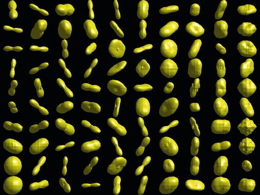
290     A. Gramfort, C. Poupon, and M. Descoteaux

dictionary. The integer k is the size of the dictionary. The noise ei ∈ Rd+ is known
to have a Rician distribution and non-central χ-distribution when using parallel
imaging [3,4]. However, for the current contribution, it will be assumed Gaussian
with mean µ ∈ Rd and diagonal covariance Σ = diag((σj2 )j=1,...,d ) ∈ Rd×d . We
denote it ei ∼ N (µ, Σ). This modeling assumption is valid for images with SNR
above 4 [3], which is the case for the DSI data used in this paper.
   The estimation procedure detailed below requires that the additive noise to
be Gaussian with unit variance. To meet this constraint, we define the whitened
data Siw = Σ−1/2 (Si − µ) so that Siw ∼ N (Dw Wi , I) where Dw = Σ−1/2 D. In
practice, µ and Σ are estimated from voxels with weak diffusion (e.g. the skull).
   In order to learn the dictionary D one needs to set priors on both D and W.
The positivity of DWI data imposes that D ! 0 and W ! 0. The dictionary is a
good model for the entire white matter but the data at a given voxel should only
be formed by a linear combination of a few DSI profiles: W should be sparse,
i.e. contain many zeros. This leads to the following minimization:

               (D     % = argmin 1 "Sw − Dw W"2Fro + λ"W"1
                $ w , W)                                                        (2)
                           D,W 2d

                         s.t. "Dk "22 " 1, D ! 0, W ! 0

The parameter λ balances the reconstruction error and the $1 regularization term
which promotes sparse coefficients W. Columns of D have unit norm to avoid
scaling ambiguity. Following [5], we use an online cyclic descent to minimize (2).
The estimated dictionary D $ is then given by D$ = Σ1/2 D $ w.

Denoising and subsampling. Given a learned dictionary D, one can estimate the
coefficients of a decomposition for a new dataset, with possibly less directions
than the original dataset used to learn D, i.e. using only a limited set of rows
of D. Let us denote I a list of sampling directions (|I| " d). Given a set of
whitened subsampled data SIw , the coefficients W can be obtained by solving:

         % = argmin 1 "SIw − DIw W"2 + δ"W"1
         W                                                     s.t. W ! 0
                                   Fro
               W   2|I|

                                                      $ = DW
where δ > 0. The full signal can then be obtained as: S    % ∈ Rd×p .

Model selection and choice of parameters. The estimation procedure involves
a few parameters, λ to learn a dictionary and δ to estimate the coefficients
given the dictionary. In order to tune these parameters we use cross-validation
exploiting the symmetry of the signal.
   Given half of the directions H (d=258 directions), a good model should be
able to predict the other half by applying a simple symmetry to the data. This
observation also allows us to estimate a full dictionary of 2d − 1 = 515 directions
using only half of the data. The minimization of (2) restricted to the data SH
      $ H ∈ Rd×k which leads to D
gives D                            $ ∈ R2d−1×k by applying a symmetry.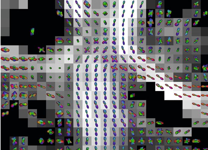
Sparse DSI: Learning DSI Structure for Denoising and Fast Imaging           291

                       a)

                      b)

Fig. 1. In green are the 258 directions H used to estimate a dictionary. a) For intra-
subject cross-validation, in red are the directions L used to estimate the coefficients
and in blue the left out directions T used to evaluate the model parameters. The white
directions V are only used for validation. b) For inter-subject cross-validation the same
color code applies. There is no validation set in this case, as the validation data is
obtained from the other subject.

   In order to assess the quality of the model without overfitting, the model selec-
tion involves two other sets of directions: L to learn W  % and T to test the recon-
struction error. The best parameters minimize this error. It is quantified with the
                                                           1         $ % 2
average root mean square error (RMSE): RMSE = p|T            | "ST − DT W"Fro . This
procedure is a principled way of choosing the parameters. Once they are set, the
model estimated can be tested on new DWI V for validation. As V has not been
used for training, RMSE obtained by different algorithms can be compared.
   In the following experiments, the parameter λ was set in a range of 5 values
(1, 0.1, 0.01, 0.001) and δ in a logarithmic grid of 15 values between 0 and 1e−6 . In
order to quantify the performance of our method, we use as baseline the solution
that consists in applying a simple symmetry to the data, as done classically [2].
We denote RMSEsym the error obtained. We report the quality of our solution as
a ratio between the two quantities: ρRMSE = RMSEsym /RMSE. A ratio above
1 indicates an improvement with respect to a symmetrization.
   The following results involve two setups. An intra-subject denoising procedure
and an inter-subject procedure where a dictionary learned on a subject is used
to estimate a full resolution DSI dataset for a new subject from only a few DWI.
See Fig. 1 for details on H, L, T and finally V used to estimate ρRMSE .
   The data consists of 2 subjects. A standard DSI acquisition mimicking [1]
was done with isotropic 2 mm spatial resolution and d = 515 DWI were ac-
quired sampling the q-space on a cubic lattice within the sphere of radius 5,
TE/TR=147ms/11.5s, BW=1680Hz/pixel, 96x96 matrix, and 60 axial slices
with a parallel reduction factor of 2, δ and ∆ were 41 and 45 ms, resulting
in a maximum q-value of qmax = 70.4 mm−1 , bmax = 6000 s/mm2 . The SNR
of the b = 0 image was 36 and the SNR of the DWI for the b = 960, 3360,
and 6000 s/mm2 datasets were estimated to 12, 7.5, and 6.5 respectively. For
the rest of this paper, acquisition of 258 directions with simple symmetry will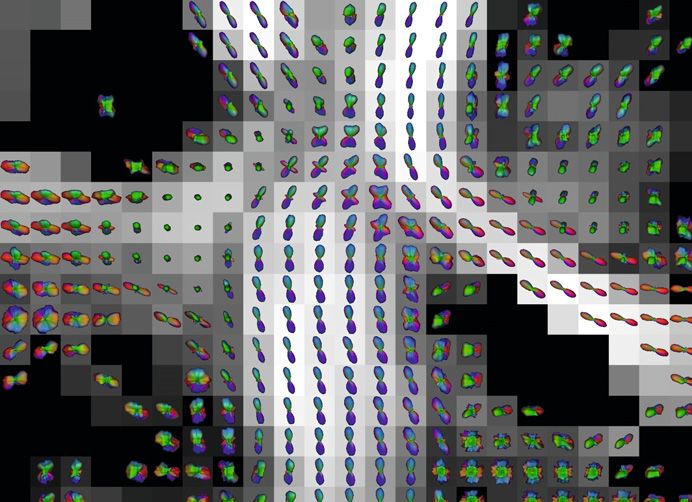
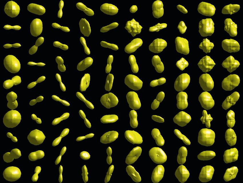
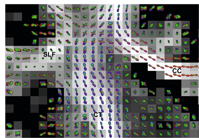
292     A. Gramfort, C. Poupon, and M. Descoteaux

be abbreviated HALF, as opposed to the FULL acquisition. Different symmetry
completion procedure are also included for comparison, either using Gaussian
smoothing with σ = 0.35 (optimal σ in our experiments) and state-of-the-art
non-Local (NL) means denoising [6]. Finally, ODFs are computed as described
above and visualized as deformed spheres with the radius proportional to Ψ (u).

3     Results
Figure 2 shows the ODFs of the learned dictionaries with 100 atoms on both
subjects. Atoms are ordered from left to right, starting at the bottom left corner
based on the variance they explain on the data. We see that most important
atoms are isotropic profiles and several single fiber structures. After approxi-
mately 30 atoms, crossing profiles appear. At the end of the dictionary, more
complex ODF profiles are also present. This behavior of the learned dictionary
is similar if we increase its size k.
   Intra-subject denoising Table 1 shows how sparse DSI reconstruction is able
to accurately reconstruct the un-measured 257 directions. It has lower RMSE
than the usual symmetry and, Gaussian and NL means denoising. Increasing
the number of atoms in the dictionary only slightly improves the accuracy on
subject 2. Moreover, Fig. 3 confirms that denoising, in general, improves the raw
DSI data. However, it can be seen that NL means and Gaussian denoising seem
to over-smooth and blur the structure of the raw data, as opposed to sparse DSI
that appear to denoise but also enhance structure. Finally, Fig. 4 overlays ODFs
in a zoom region of this slice, corresponding to the centrum semiovale where
corpus callosum (CC) crosses with the corticospinal tract (CT) and superior
longitudinal fasciculus (SLF). Single, two and three fiber crossings can be seen.
One can appreciate how sparse DSI is able to recover ODF profiles as sharp as
the FULL raw and NL means/Gaussian denoised DSI.
   Inter-subject undersampling One can push sparse DSI and attempt to perform
DSI estimation and ODF reconstruction from undersampled q-space data. The
compressed sensing literature teaches us that the ”sensing” strategy is crucial for
optimal reconstructions. It is beyond the scope of this paper to explore optimal
undersampling strategies. Here, we undersampled 1 measurement out of N from
the Cartesian direction indices, which preserves a uniform Cartesian sampling.

Fig. 2. ODFs computed from the learned dictionaries on the 2 subjects (100 atoms
and inter-subject cross-validation). Left (resp. right) is for subject 1 (resp. 2).
Sparse DSI: Learning DSI Structure for Denoising and Fast Imaging   293

Table 1. Intra-subject denoising. ρRM SE between simple DSI symmetry, Gaussian
smoothing, NL means and sparse DSI denoising. Sparse DSI reconstruction gives the
best performance on the validation data.

 Methods Gaussian NL means                    Sparse                               DSI
          σ = 0.35         k = 100 k = 169 k = 225 k                               = 400 k = 900 k = 1600
 Subject 1 1.16     1.19     1.31    1.31    1.31                                  1.31    1.31    1.31
 Subject 2 1.13     1.16     1.28    1.25    1.23                                  1.30    1.30    1.29

                                                     Sparse DSI   Raw DSI   NL means       Gaussian
    b = 6000 s/mm2 b = 3360 s/mm2 b = 960 s/mm2
    q = (−5, 0, 0) q = (−3, −2, −1) q = (0, 0, −2)

Fig. 3. Denoising the raw data DSI with our sparse DSI technique versus state-of-the-
art non-local means (NLM) and Gaussian (optimal σ = 0.35) denoising.

   Figure 5 shows the RMSE ratio between simple HALF DSI with symmetry
and sparse DSI as a function of number of measurements. We also show the ODF
field in Fig. 6 as a function of number of measurements. First, it is amazing to see
that a learned DSI dictionary of a subject can be used to perform undersampled
DSI on a different subject. It means that both dictionaries in Fig. 2 look similar
and quantitatively yield comparable performances. Of course, as undersampling
decreases, the overall field of ODF seems more noisy but the overall RMSE
remains acceptable. At a total of 37, 29, and 21 measurements, we become worst
than NL means, Gaussian smoothing and simple symmetry DSI in terms of
RMSE. On the other hand, we observe that ODF profiles are degraded sooner
as a function of undersampling. Note that the structured voxels with single fiber
orientation in the CC, CT and SLF are well preserved all the way down to
29 measurements. However, although crossings are found for all undersampling,
ODF peaks in crossing areas become less accurate below 58 measurements.
294                 A. Gramfort, C. Poupon, and M. Descoteaux

Sparse DSI (k=100)                    FULL DSI       FULL NL means         FULL Gauss

Sparse DSI (k=400)                    HALF DSI       HALF NL means         HALF Gauss

Fig. 4. Full (d = 515) DSI vs. Half DSI (d = 258) with respect to simple symmetry,
Gaussian (σ = 0.35), NL means and sparse DSI denoising of subject 1 (k atoms).

              1.3

              1.2
Error ratio

              1.1
                                                                 Gaussian σ = 0.35 brain1
                                                                 NL−means brain1
               1                                                 Gaussian σ = 0.35 brain1
                                                                 NL−means brain2
                                                                 Baseline with symmetry
              0.9                                                Sparse DSI brain1/brain1
                                                                 Sparse DSI brain1/brain2
                                                                 Sparse DSI brain2/brain2
              0.8
                                                                 Sparse DSI brain2/brain1
                    6 18   37    58      86 103115 129 147      172      206            258
                                           # of measurements used

Fig. 5. Reconstruction error ratios for intra and inter-subject settings as a function
of the number of measurements (k=100 atoms). brain1/brain1 is for the intra-subject
case while brain1/brain2 is the inter-subject (Atoms learned on subject 1 and used the
estimate the full DSI data of subject 2 using only a few measurements).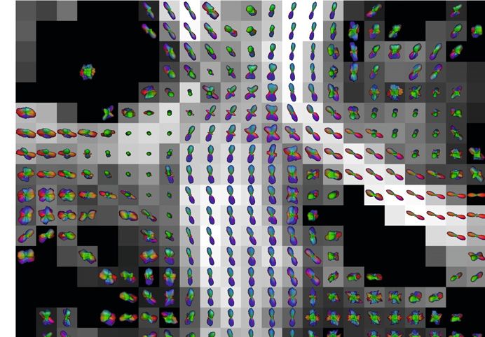
Sparse DSI: Learning DSI Structure for Denoising and Fast Imaging 295
258 129 58
43 37 29
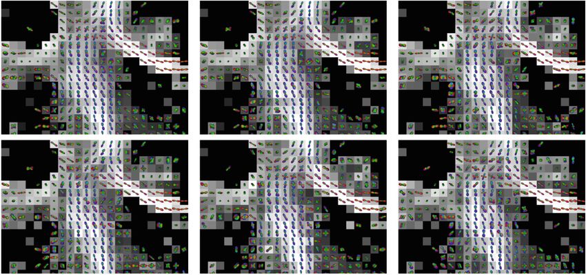
Fig. 6. Undersampled sparse DSI using learned dictionary from subject 1 to reconstruct
DSI signal and diffusion ODFs of subject 2. In white is the number of measurements.
4 Discussion and Conclusion
Sparse coding applied to DSI data reveals the latent structure of the white mat-
ter. Sparse coding is however not compressed sensing (CS), as done for DSI
in [7]. Although our technique attempts to infer full DSI data from undersam-
pled acquisitions, there is no “sensing” in the technique. The idea is to learn the
structure of raw DWI from a full DSI acquisition to either, denoise the DSI data,
or use the learned dictionary of DSI profiles to perform undersampled DSI acqui-
sitions and reconstructions. While [7,8,9] fix a priori the sparse representation of
the data (e.g. spherical ridgelets) we propose here to estimate it. The technique
proposed is attractive thanks to its little modeling assumptions and its limited
number of parameters that can be estimated by cross-validation.
The key benefit of our method is its ability to perform denoising across all the
DWI channels jointly, consequently enhancing the image quality in particular
for noisy high b-values. While the technique of [10] uses DW images within a
certain cone around the DW image being denoised, we propose to estimate the
underlying structure from all directions and b-values. This is made possible by
a proper whitening of the data in order to combine in the estimation multiple
images corrupted by different noise levels.
Results have showed that with just half of the data (258 DWI), we can better
predict the other 257 DWI than the classic symmetry procedure. This statement
also holds even if we use as little as 40 q-space measurements. Our sparse DSI
technique performs better than symmetrizing, Gaussian denoising or state-of-
the-art NL means. Finally, beyond denoising, we have showed that learning the
dictionary from one subject can be used to reconstruct full DSI dataset from an
undersampled acquisition of a different subject. From now on, we could acquire
around 40 measurements on new subjects and use the learned dictionaries to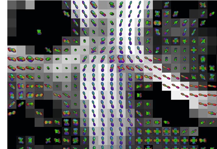
296     A. Gramfort, C. Poupon, and M. Descoteaux

reconstruct a full DSI data. Hence, we can have fast acquisitions to obtain high
resolution DSI data. Therefore, DSI can be done at the price of HARDI!
   Future work will be dedicated at optimizing the dictionary learning to enhance
ODF reconstruction and also to find optimal sub-sampling strategies.

References
 1. Wedeen, V.J., Hagmann, P., Tseng, W.Y.I., Reese, T.G., Weisskoff, R.M.: Mapping
    complex tissue architecture with diffusion spectrum magnetic resonance imaging.
    Magnetic Resonance in Medicine 54(6), 1377–1386 (2005)
 2. Hagmann, P., Cammoun, L., Gigandet, X., Meuli, R., Honey, C.J., Wedeen, V.J.,
    Sporns, O.: Mapping the structural core of human cerebral cortex. PLoS Biology
    6(7), e159 (2008)
 3. Sijbers, J., den Dekker, A.J., Audekerke, J.V., Verhoye, M., Dyck, D.V.: Estimation
    of the noise in magnitude MR images. Magnetic Resonance Imaging 16(1), 87–90
    (1998)
 4. Koay, C.G., Özarslan, E., Basser, P.J.: A signal transformational framework for
    breaking the noise floor and its applications in MRI. Journal of Magnetic Reso-
    nance 197(2), 108–119 (2009)
 5. Mairal, J., Bach, F., Ponce, J., Sapiro, G.: Online learning for matrix factorization
    and sparse coding. Journal of Machine Learning Research 11, 19 (2010)
 6. Coupé, P., Manjón, J.V., Gedamu, E., Arnold, D., Robles, M., Collins, D.L.: Robust
    rician noise estimation for MR images. Medical Image Analysis 14(4), 483–493
    (2010)
 7. Menzel, M.I., Tan, E.T., Khare, K., Sperl, J.I., King, K.F., Tao, X., Hardy, C.J.,
    Marinelli, L.: Accelerated diffusion spectrum imaging in the human brain using
    compressed sensing. Magnetic Resonance in Medicine 66(5), 1226–1233 (2011)
 8. Landman, B.A., Bogovic, J.A., Wan, H., ElShahaby, F.E.Z., Bazin, P.L., Prince,
    J.L.: Resolution of crossing fibers with constrained compressed sensing using dif-
    fusion tensor MRI. NeuroImage 59(3), 2175–2186 (2012)
 9. Michailovich, O., Rathi, Y., Dolui, S.: Spatially regularized compressed sensing for
    high angular resolution diffusion imaging. IEEE Transactions on Medical Imag-
    ing 30(5), 1100–1115 (2011)
10. Tristán-Vega, A., Aja-Fernández, S.: DWI filtering using joint information for DTI
    and HARDI. Medical Image Analysis 14(2), 205–218 (2010)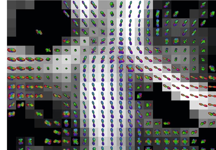
You can also read