SPECTRA, IMAGES, SIMPLE FUNCTIONS, AND DENSITY FUNCTIONS - IEEE ...

Page created by Ronnie Stanley
 
CONTINUE READING
SPECTRA, IMAGES, SIMPLE FUNCTIONS, AND DENSITY FUNCTIONS - IEEE ...
SPECTRA, IMAGES, SIMPLE FUNCTIONS, AND DENSITY FUNCTIONS

                                                           Nathan Hagen

    Utsunomiya University, Department of Optical Engineering, Utsunomiya, Tochigi 321-8585 Japan

                          ABSTRACT                                    meaning of optical measurement. As a result, the relevance to
                                                                      spectrometry of the distinction between simple functions and
When working with spectra that represent optical power or
                                                                      density functions may not seem immediately obvious, but we
photon number, we must be very careful with our units. Since
                                                                      will show that while it can often be ignored in standard 2D
most spectral transformations are nonlinear, the transforma-
                                                                      imaging, it often cannot be ignored in spectrometry without
tion Jacobian produces a nonlinear distortion of the spectrum.
                                                                      causing severe errors.
A surprising number of researchers ignore these issues and
                                                                          One field where this distinction is introduced early on to
misrepresent their spectra in their publications.
                                                                      students, and hammered into their heads regularly in the cur-
    Index Terms— spectrum, nonlinear transformation, den-             riculum, is probability theory, where the two are labelled as
sity functions, distortion, Jacobian                                  mass functions and density functions. Here I will refer to
                                                                      them as simple functions and density functions. While math-
                    1. INTRODUCTION                                   ematicians who work in probability theory have a habit of
                                                                      saying that measure theory, Stieltjes integrals, and similar
Most researchers, even in our field where they really should          20th century tools of mathematics are required tools in or-
know better, think of a spectrum as a simple graph. One can           der to work with density functions,[3] these are unnecessary
point to a location on a reflectivity spectrum curve and say          for practical work. Physicists have been working with density
something like “look here — the reflectivity at λ = 600 nm is         functions long before measure theoretic tools were developed,
0.5.” If light reflects first from one surface and then another,      and realize that one need only pay close attention to units and
then we can simply multiply the two reflectance spectra to-           to the physical meaning of the quantities being manipulated.
gether to get the overall reflectance of the combination. How-
ever, we cannot do this for an irradiance spectrum. We cannot                  2. WAVELENGTH ↔ WAVENUMBER
place a finger on a irradiance spectrum and say something like                       TRANSFORMATIONS
“see, the irradiance here at λ = 600 nm is 10 W m−2 ”. Unlike
the reflectance spectrum, the irradiance spectrum does not de-        The Planck blackbody function provides a useful demonstra-
fine the irradiance at a single point. Rather, it defines the dif-    tion for how the units we use can affect the shape of the spec-
ferential irradiance with respect to the wavelength, as implied       tra we draw. The most common representation for the func-
by the units 10 W m−2 nm−1 , so that the irradiance value is          tion is to calculate the spectral radiance in flux units of Watts
given by integrating the spectrum over a specified range. As a        on a wavelength axis, using the expression
result, it also makes no sense to multiply two irradiance func-
tions together.                                                                                2hc2     1         
                                                                                    Le (λ) =                         .
     While the distinction between these two forms of spectra                                   λ5 ehc/(λkbT ) − 1
can be ignored in many circumstances, there are also many             Here, L is the spectral radiance [W m−2 sr−1 µm−1 ], with the
situations in which they cannot, and inattention to this de-          subscript “e” indicating the use of energy-based flux units.
tail has produced errors in work published throughout our             The constants are the speed of light c [m/s], kB Boltzmann
field. It is, for example, partly responsible for the surpris-        constant [J/K], and Planck constant h [J s], while T [K] is the
ingly persistent fallacy that the human eye’s sensitivity is          temperature parameter, and λ [µm] is the wavelength. For the
matched to the peak of the Sun’s radiance spectrum.[1] The            Planck blackbody function represented in a different domain
fields of physics and engineering that use measurements of            such as wavenumber or frequency, see Tab. 1.
optical spectra, like most other areas of physics, sometimes              Next we look at what happens when we try to trans-
forget to make clear distinctions between simple functions            form the blackbody spectrum from a wavelength basis to
and density functions. Very few textbooks even discuss the            a wavenumber basis. Here we will use the definition of
issue,[2] despite its fundamental importance in explaining the        wavenumber as σ = 1/λ. (A common alternative definition
    This work was supported by JSPS KAKENHI Grant JP20K04516 Grant-   of wavenumber is k = 2π/λ.) Any legitimate transforma-
in-Aid for Scientific Research.                                       tion of the spectrum must preserve the overall energy (or
1.0
                                                         (a)                                                                                         frequency [THz] or energy [eV]. Since these units are pro-
                                                                                                                                                     portional to wavenumber, however, they only change the axis
        normalized spectral radiance

                                                  0.8

                                                                                                                                                     labels and not the shape of the curve. These four options for
                                                  0.6                                                                                                the abscissa are what we can call the “density units” of the
                                                  0.4
                                                                                                                                                     spectrum. Table 1 gathers together a set of Planck function
                                                                                         W / (m2 sr μm)                                              representations for each different choice of domain.
                                                                                         (photons s-1) / (m2 sr μm)
                                                  0.2
                                                                                         W μm / (m2 sr)
                                                                                         (photons s-1 μm) / (m2 sr)

                                                  0.0                                                                                                           3. POWER ↔ PHOTON NUMBER
                                                                 400             600            800               1000                 1200
                                                                                          wavelength [nm]                                                            TRANSFORMATIONS
                                                                                         wavelength [μm]
                                                                1 .0   0 .7 5                 0 .5             0 .4                           0 .3   While the wavelength-wavenumber transformation of the
    spectral radiance [a.u. ∝ W μm, or phot μm]

                                                  1 .0
                                                                                                                                 2
                                                                                                                       W μm / (m sr)
                                                                                                                                                     spectrum is widely recognized, and mistakes regarding it are
                                                  0 .8
                                                                                                                       (photons s-1 μm) / (m2 sr)
                                                                                                                                                     not so common in the literature, the transformation of flux
                                                                                                                                                     units from power (Watts) or photon number is abused almost
                                                  0 .6
                                                                                                                                                     everywhere. Since the energy of a photon is wavelength
                                                  0 .4
                                                                                                                                                     dependent, transforming the ordinate of the spectrum from
                                                                                                                                                     Watts to photons/sec causes a shift in the shape of a spectrum.
                                                  0 .2                                                                                               As a result, it matters very much which ordinate we choose.
                                                          (b)                                                                                        In Fig. 1, two of the curves are representations for the Planck
                                                  0 .0
                                                                1 .0            1 .5           2 .0             2 .5                 3 .0
                                                                                       wavenumber [μm-1]
                                                                                                                                                     blackbody curve using an ordinate proportional to photon
                                                                                                                                                     number rather than Watts. Since the number of photons per
Fig. 1. (a) The Planck blackbody spectrum for a 5770 K                                                                                               unit energy is larger at longer wavelengths, the transforma-
source (an approximation to the above-atmosphere solar ra-                                                                                           tion from Watts to photons lifts up the long-wavelength end
diance spectrum), normalized to a peak value of 1. The                                                                                               of the spectrum — shifting the peak of the curve to the red.
black and blue curves are calculated in wavelength space,                                                                                                The majority of detectors that we use in research these
while the red and green curves are calculated in wavenum-                                                                                            days are integrating sensors, such as the CCD and CMOS de-
ber space, then re-sampled onto a linear wavelength grid in                                                                                          tector arrays used in imaging and spectrometry, as well as
order to demonstrate the change in shape. (b) The red and                                                                                            cryo-cooled infrared detector arrays. The digital number that
green curves calculated in a linear wavenumber space.                                                                                                these sensors return is proportional to the number of photo-
                                                                                                                                                     electrons collected by the sensor during the integration pe-
                                                                                                                                                     riod. As a result, if we plot data from a digital spectrometer,
photon number) of the integrated spectrum. With this con-                                                                                            we should almost always choose the spectrum ordinate to be
straint, we can either work directly with infinitesimals to                                                                                          proportional to photon number and not Watts.
write dσ = −dλ/λ2 or equivalently work with the integral                                                                                                 The second category of detectors are flux sampling sen-
directly to write                                                                                                                                    sors, which include photodiodes and bolometers (among oth-
   Z                                              λ2                     Z      σ(λ2 )                                                               ers). The digital number returned by these detectors is propor-
                                                                                     dλ
                                                         L(λ) dλ =                       L(λ(σ))
                                                                                         dσ                                                          tional to the instantaneous optical power incident on the face
           λ1                                                        σ(λ1 )          dσ                                                              of the sensor. Thus, if we plot data from a spectrometer us-
                                                           Z σ(λ2 )                     Z σ2
                                                                                                                                                     ing a microbolometer detector array, the appropriate ordinate
                                                         =          L(λ(σ)) (−λ2 ) dσ =      L(σ) λ2 dσ                                              would be proportional to Watts.
                                                            σ(λ1 )                                                        σ1
                                                                                                                                                         The largest number of mistakes occur when authors draw
where the last line uses the negative sign to swap the order of                                                                                      a spectrum measurement and write “intensity [a.u.]” for the
integration. The factor of λ2 inside the integral tells us that the                                                                                  ordinate of the plot. If the abscissa is labelled as wavelength
resulting curve will have a different shape, as we see in Fig. 1,                                                                                    (or wavenumber), then we can infer that the intensity must
where the above transformation is indicated by the black and                                                                                         also be represented in wavelength (or wavenumber) space. If
red curves. Since the two curves are plotted together on the                                                                                         the writer is discussing a modern detector array as the source
same linear wavelength abscissa, one might justifiably feel                                                                                          of the measurements, then we can also infer that the ordi-
that doing this for the wavenumber-space representation is il-                                                                                       nate must be proportional to photon number. In older publi-
legitimate. Indeed, drawing the curve this way does not pre-                                                                                         cations, especially before the 1990s, almost all sensors were
serve the energy of the integral. It does, however, preserve the                                                                                     flux-sampling, and so we can infer that the ordinate will be
shape of the function, so that we can demonstrate changes in                                                                                         proportional to optical power. However, the momentum of
the location of the peak.                                                                                                                            history has been such that many modern authors persist in dis-
    In addition to the wavelength and wavenumber axes, other                                                                                         cussing radiometric units of optical power while using CCD
common representations of optical spectra use abscissae of                                                                                           and CMOS integrating sensor arrays. The result is a misla-
1.0
                                                                                                                                                                                                                       (a)

                                                                               intensity [a.u. ∝ phot/μm]
                                                                                                            0.8

                                                                                                            0.6
                                                                                                                                                                                                            (uniformly sampled)
                                                                                                            0.4

                                                                                                            0.2

                                                                                                            0.0
                                                                                                                  400          500         600        700       800                                         900      1000
                                                                                                                                                  wavelength [nm]

                                            1.0                                                                                                                                           1.0
                                                                                                                                           (b)                                                                                                                             (c)
          intensity [a.u. ∝ phot/channel]

                                                                                                                                                           intensity [a.u. ∝ phot/μm-1]
                                            0.8                                                                                                                                           0.8

                                            0.6                                                                                                                                           0.6
                                                                                                                    (non-uniformly sampled)                                                                                                                (uniformly sampled)

                                            0.4                                                                                                                                           0.4

                                            0.2                                                                                                                                           0.2

                                            0.0                                                                                                                                           0.0
                                                   1.0     1.2   1.4   1.6    1.8     2.0                                2.2         2.4     2.6                                                    1.0      1.2     1.4     1.6    1.8     2.0            2.2       2.4    2.6
                                                                       wavenumber [μm-1]                                                                                                                                     wavenumber [μm-1]

Fig. 2. (a) A spectrum measured with a modern grating spectrometer, so that the appropriate units for the ordinate are propor-
tional to phot/µm. A low-resolution discrete spectrum is superimposed over the measured spectrum. (b) The spectrum shown in
(a) resampled onto a nonuniform wavenumber grid. The nonuniform sampling is not clear when the samples are tightly spaced
(grey curve) but are obvious in the low-resolution discrete spectrum (black lines). (c) If we interpolate the spectrum from (a)
onto a uniformly-sampled wavenumber grid, we need to rescale the individual channel bins in order to conserve overall photon
count.

                                                                       Table 1. Planck blackbody expressions in different domains.[6]
                                                         Spectrum variable                                                     Quantum flux                                                                           Optical power
                                                                                                                                                                                                                          2
                                                                                                                                                                                                                                                
                                                         Wavelength λ:                                                  Lq (λ) = λ2c4 ehc/(λk1 bT ) −1                                                         Le (λ) = 2hc
                                                                                                                                                                                                                         λ5     e
                                                                                                                                                                                                                                       1
                                                                                                                                                                                                                                  hc/(λk bT ) −1
                                                                                                                        [photon s−1 m−2 sr −1
                                                                                                                                         µm ]
                                                                                                                                              −1
                                                                                                                                                                                                              [W m−2 sr−1 µm−1
                                                                                                                                                                                                                               ]                             
                                                                                                                                           2ν 2                                           1                                   2hν 3                1
                                                         Frequency ν = c/λ:                                             Lq (ν) =            c2      ehν/(kbT ) −1
                                                                                                                                                                                                               Le (ν) =        c2         ehν/(kbT ) −1
                                                                                                                        [photon s−1 m−2 sr−1 Hz−1 ]                                                            [W m−2 sr−1 Hz−1 ]
                                                                                                                                                  2cσ 2                                                                          2hc2 σ 3
                                                         Wavenumber σ = 1/λ:                                            Lq (σ) =           ehcσ/(kbT ) −1
                                                                                                                                                                                                               Le (σ) =       ehcσ/(kbT ) −1
                                                                                                                        [photon s−1 m−2 sr −1
                                                                                                                                         cm]                                                                 [W m−2 sr−1 cm]                                  
                                                                                                                                           ck2                                            1                                   h̄c2 k3                  1
                                                         Wavenumber k = 2π/λ:                                           Lq (k) =           4π 3     eh̄ck/(kbT ) −1
                                                                                                                                                                                                               Le (k) =         4π 3          eh̄ck/(kbT ) −1
                                                                                                                        [photon s−1 m−2 sr−1
                                                                                                                                           cm]                                                               [W m−2 sr−1 cm]                              
                                                                                                                                           2E 2                                               1                                   2E 3             1
                                                         Energy E = hc/λ (eV):                                          Lq (E) =           c2 h3      eE/(kbT ) −1
                                                                                                                                                                                                               Lp (E) =           c2 h3       eE/(kbT ) −1
                                                                                                                        [photon s−1 m−2 sr−1 eV−1 ]                                                            [W m−2 sr−1 eV−1 ]

                                                                                                                                                                                          0.5
                                                                                                                                                          normalized intensity

                                                                                                                                                                                          0.4

                                                                                                                                                                                          0.3

                                                                                                                                                                                          0.2

                                                                                                                                                                                          0.1

                                                                                                                                                                                          0.0
                                                                                                                                                                                                  450          500      550       600                      650
                                                                                                                                                                                                                  wavelength (nm)

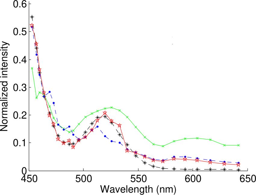
                                                  Fig. 3. (a) Original figure from Ref. [7]. (b) The black curve copied and (red, blue) transformed.
belling of the axes, or a distortion of the spectrum shape.
                                                                   Table 2. The Wien displacement law for peak wavelength,
     Even Soffer & Lynch, who have written the article [1]
                                                                   expressed in different domains.[8, 9]
most often cited regarding the fallacy of the eye’s opti-
                                                                    Spectrum variable           Quantum flux          Optical power
mization to green, focus their discussion almost entirely on
                                                                                                        3669.7 µm K            2897.8 µm K
the wavelength-wavenumber transformation rather than the            Wavelength λ:              λw =          T
                                                                                                                      λw =          T
energy-photon transformation, even though the meaning of            Frequency ν = c/λ:         λw   =   9028.4 µm K
                                                                                                                      λw   =   5099.4 µm K
                                                                                                             T                      T
the abscissa transformation is unclear in the case of the eye.      Wavenumber σ = 1/λ:        λw   =   9028.4 µm K
                                                                                                                      λw   =   5099.4 µm K
                                                                                                             T                      T
It is clear, however, that the ordinate of the radiance spectrum    Wavenumber k = 2π/λ:       λw   =   9028.4 µm K
                                                                                                                      λw   =   5099.4 µm K
                                                                                                             T                      T
should be represented in photons rather than energy, since the      Energy E = hc/λ (eV):      λw   =   9028.4 µm K
                                                                                                                      λw   =   5099.4 µm K
                                                                                                             T                      T
retina is a quantum detector and not a power detector.[4, 5]
     So far the discussion has focused on continuous represen-
tations of spectra. For laboratory measurements, however,          tion such that the highest channel value in the spectrum is
what we obtain are discrete functions. Discrete representa-        unchanged. Each curve is also drawn together with its im-
tions give us extra flexibility because the spectra have already   plied channel rectangles. Whereas the correct transformation
been integrated across the passband of the individual spectral     cannot be determined from the authors’ original figure, using
channel. If we transform the spectrum from one domain to an-       channel rectangles preserves the concept that any transforma-
other, we need only change the width of each individual chan-      tion will preserve the integral under the curve, and makes it
nel by the appropriate amount without having to rescale the        easier to choose the correct transformation. As we can see
measured data. Figure 2 gives an example of this. Figure 2(a)      from the figure, the difference in shapes between the three
shows a spectrum measured with a grating spectrometer, so          spectra is clear enough to indicate a visible color difference
that the individual spectral channels are approximately uni-       to our eyes, and a significant difference in any error metric
formly sampled in wavelength — that is, the channel bins are       used to compare results. Note that the sudden difference be-
all approximately the same width. As a result, the ordinate of     tween the original curve and transformed curves at the third
the figure can be written with units proportional to phot/µm or    point from the left is due to an odd change in the sampling
phot/channel, whichever the user prefers. Figure 2(b) shows        distance between the points there.
the same spectrum in which the edges of the spectral channels
have been translated to the wavenumber domain, while the           4. THE EFFECT OF DOMAIN CHOICE ON WIEN’S
values of the bins have been left unchanged. This of course                           LAW
preserves the overall photon number, but it produces nonuni-
form sampling — the individual channels are no longer the          As illustrated in Fig. 1, one of the striking changes caused by a
same width. Here the only appropriate way to write the ordi-       change in the flux units or density units in which we represent
nate would be with units proportional to phot/channel. If we       a spectrum is that the peak of the blackbody spectrum. For a
want to interpolate this spectrum onto a uniformly sampled         spectrum represented in W/µm, the expression governing the
grid, then we need to re-scale the heights of the individual       location of this peak is
discrete channels according to the Jacobian of the transforma-
tion (dλ → −λ2 dσ), the result of which is shown in Fig. 2(c).                       λw = (2897.8 µm K) T −1 .
Here the ordinate can now be written with units proportional
to phot/µm−1 or phot/channel.                                      Thus, when we approximate the solar spectrum with a black-
     Although it is perhaps unfair to single out any single au-    body spectrum of a 5770 K object, we find that the Wien peak
thor for violating these rules, it is useful to have an exam-      is located at a wavelength of 502 nm. Table 2 gives expres-
ple demonstrating how normalization errors affect published        sions for the Wien law for blackbody spectra expressed in
data. Figure 3(a) shows a figure taken from the literature, us-    other domains. For a spectrum represented in photons/µm, the
ing a normalized ordinate, and nonuniformly sampled points         solar Wien peak shifts to 636 nm. If we switch to wavenum-
on the abscissa.[7] The authors use this figure to compare         ber densities, then the solar Wien peaks become 884 nm (for
their reconstructed spectra to measurements with a standard        W µm) and 1565 nm (for photons µm). Figure 4 illustrates the
laboratory spectrometer, and state that they scale the mea-        changes in the spectral shapes and peak locations as a func-
surements from the lab spectrometer by normalizing them            tion of temperature and domain.
with the “energies” at each point. This is not the correct
way to transform data taken with a photon integrating de-          5. NONLINEAR TRANSFORMS IN IMAGING DATA
tector in order to compare to another photon-integrating sen-
sor, but perhaps the authors meant only normalization by the       While spectral transformations are often nonlinear, such as
areas. Figure 3(b) replicates the black curve from (a) but         the wavelength-wavenumber and energy-photon transforms,
rescales it according to the channel widths (red curve) and        most image transformations are linear. When distorting im-
total channel energies (blue curve), followed by normaliza-        ages, or mapping 3D surfaces onto 2D, the transformations
×1021
                                                                        45                                                                                                                                        1.8

                                                                                                                                                            spectral radiance (photons s-1 m-2 sr-1 μm-1)
                                                                        40
                                                                                                     400K
                                                                                                                                           (a)                                                                    1.6                                            400K
                                                                                                                                                                                                                                                                                             (b)
                                  spectral radiance (W m-2 sr-1 μm-1)   35                                                                                                                                        1.4
                                                                                                                                                                                                                                                  Wien
                                                                        30               Wien                                                                                                                     1.2                             curve
                                                                                         curve
                                                                        25                                                                                                                                        1.0                                               350K
                                                                        20
                                                                                                            350K                                                                                                  0.8

                                                                        15                                                                                                                                        0.6                                                       300K
                                                                        10                                         300K                                                                                           0.4
                                                                                                                                                                                                                                                                                    250K
                                                                         5                                                    250K                                                                                0.2

                                                                        0                                                                                                                                         0.0
                                                                                   5                    10                      15                20                                                                                  5                   10                   15                 20
                                                                                                        wavelength (μm)                                                                                                                                   wavelength (μm)

                                                                                                        wavelength (μm)                                                                                                                                   wavelength (μm)
                                                                             100   20           10       7           5               4           3                                                                          100      20           10       7          5             4              3
                                                0.40                                                                                                                                  ×1019

                                                                                                                                           (c)
                                                                                                                                                                                                                  3.0

                                                                                                                                                                    spectral radiance (photons s-1 m-2 sr-1 cm)
                                                                                            400K
                                                 0.35                                                                                                                                                                                      400K
                                                                                                                                                                                                                                                                                              (d)
          spectral radiance (W m-2 sr-1 cm)

                                                                                                                                                                                                                  2.5
                                                0.30                                      Wien
                                                                                          curve                                                                                                                                           350K
                                                 0.25                                                                                                                                                             2.0
                                                                                               350K
                                                0.20                                                                                                                                                              1.5                     300K
                                                 0.15                                     300K
                                                                                                                                                                                                                  1.0
                                                                                                                                                                                                                                      250K
                                                0.10                                    250K
                                                                                                                                                                                                                  0.5
                                                 0.05                                                                                                                                                                             Wien
                                                                                                                                                                                                                                  curve
                                                0.00                                                                                                                                                              0.0
                                                                                                                                                                                                                  -1
                                                                             0     500         1000         1500       2000      2500    3000   wavenumber (cm )                                                        0            500         1000     1500       2000       2500       3000   wavenumber (cm-1)

                                                                                                                                                frequency (THz)                                                                                                                                   frequency (THz)

Fig. 4. The Planck blackbody function and Wien law, for various temperatures, in the domains proportional to (a) W/µm, (b)
photons/µm, (c) W cm, and (d) photons cm.

                          A                                                                                        A                                                                                                                                           7. REFERENCES

                                                                                                                                                                                                                        [1] B. H. Soffer and D. K. Lynch, “Some paradoxes, errors,
                                                                                   B                                                 B
                                                                                                                                                                                                                            and resolutions concerning the spectral optimization of
                                                                                                                                                                                                                            human vision,” Am. J. Phys. vol. 67: pp. 946–953, 1999.
    Fig. 5. Distortion of images is a nonlinear transform.                                                                                                                                                              [2] C. F. Bohren and E. E. Clothiaux, Fundamentals of Atmo-
                                                                                                                                                                                                                            spheric Radiation. Wiley, 2006.
                                                                                                                                                                                                                        [3] G.-C. Rota, “Ten lessons I wish I had learned before
are often nonlinear, so that the same warnings that we dis-                                                                                                                                                                 teaching differential equations,” in Meeting of the Math.
cussed above for spectra apply for images as well. Figure 5                                                                                                                                                                 Assoc. of Amer. at Simmons College (1997).
gives a simple example of a distortion mapping. In the case                                                                                                                                                             [4] A. Rose, “The sensitivity performance of the human eye
of images, the ordinate is typically irradiance [W/m2 ], and so                                                                                                                                                             on an absolute scale,” J. Opt. Soc. Am. vol. 38: pp. 196–
it is the 2D integral over the spatial dimension that gives us                                                                                                                                                              208, 1948.
the energy value, or photon number, that we must conserve in
                                                                                                                                                                                                                        [5] R. C. Jones, “Quantum efficiency of human vision,” J.
order to retain the correct brightness everywhere in the image.
                                                                                                                                                                                                                            Opt. Soc. Am. vol. 49: pp. 645–653, 1959.
                                                                                                                                                                                                                        [6] E. L. Dereniak and G. D. Boreman, Infrared Detectors
                                                                                                                                                                                                                            and Systems. Wiley-Interscience, 1996.
                                                                                       6. CONCLUSION                                                                                                                    [7] L. Wang et al., “High-speed hyperspectral video acquisi-
                                                                                                                                                                                                                            tion by combining Nyquist and compressive sampling”,
Although it is rare for textbooks to call attention to the distinc-                                                                                                                                                         IEEE Patt. Anal. Mach. Intel. vol. 41: pp. 857–870
tion between simple functions and density functions (Ref. [2]                                                                                                                                                               (2019).
being a rare exception), we should be aware of the distinc-                                                                                                                                                             [8] M. A. Heald, “Where is the “Wien peak”?” Amer. J. Phys.
tion between the two, and for most of us, we should make                                                                                                                                                                    vol. 71: pp. 1322–1326, 2003.
an effort to move away from using Watts when discussing                                                                                                                                                                 [9] S. M. Stewart, “Blackbody radiation functions and poly-
measurements taken with integrating sensors. For prism spec-                                                                                                                                                                logarithms,” J. Quant. Spect. Rad. Trans. vol. 113:
trometers or tunable filter spectrometers, in which the spectral                                                                                                                                                            pp. 232–238, 2012.
bins are nonuniformly spaced, being careful with these trans-
formations is a necessity.
You can also read