Comparative Study between Fuzzy Logic and Interval Type-2 Fuzzy Logic Controllers for the Trajectory Planning of a Mobile Robot
←
→
Page content transcription
If your browser does not render page correctly, please read the page content below
Engineering, Technology & Applied Science Research Vol. 11, No. 2, 2021, 7011-7017 7011
Comparative Study between Fuzzy Logic and Interval
Type-2 Fuzzy Logic Controllers for the Trajectory
Planning of a Mobile Robot
Boucetta Kasmi Abdelouaheb Hassam
Department of Electronics Department of Electronics
Laboratory of Intelligent Systems Laboratory of Intelligent Systems
University Ferhat Abbas Setif 1 University Ferhat Abbas Setif 1
Setif, Algeria Setif, Algeria
boucetta.kasmi@univ-setif.dz abdelhassam@univ-setif.dz
Abstract-In this study, Fuzzy Logic (FL) and Interval Type-2 FL of the robot in a complex environment is determined, it must be
(IT-2FL) controllers were applied to a mobile robot in order to capable of following it [6]. The generated trajectory must take
determine which method facilitates navigation and enables the into account the environmental and kinematic constraints of the
robot to overcome real-world uncertainties and track an optimal moving object [7-8]. To tackle these difficulties and to enable a
trajectory in a very short time. The robot under consideration is large number of parameters to be managed, a new control
a non-holonomic unicycle mobile robot, represented by a strategy is proposed, which is broken down into weakly
kinematic model, evolving in two different environments. The coupled units whose interactions are limited and perfectly
first environment is barrier-free, and moving the robot from an controlled in a distributed manner. The purpose is to develop
initial to a target position requires the introduction of a single robots that can move safely in unstructured environments,
action module. Subsequently, the same problem was approached
in an environment closer to reality, with objects hindering the
despite any unforeseen changes.
robot's movement. This case requires another controller, called The main problem of navigation of mobile robots can be
obstacle avoidance. This system allows the robot to reach broken down into three sub-problems: reaching the target,
autonomously a well-defined target by avoiding collision with avoiding obstacles, and tracking an optimal trajectory in a very
obstacles. The robustness of the structures of the defined short time. To reach the target, we can indicate the trajectory to
controllers is tested in Matlab simulations of the studied the robot by employing stable techniques based on the search
controllers. The results show that the IT-2FL controller performs for optimal trajectories. However, since the environments are
better than the FL controller.
rarely predictable, it makes little sense to provide the robot
Keywords-Interval Type-2 Fuzzy Logic (IT2-FL); Fuzzy Logic with a planned trajectory. Obstacle avoidance has often been
(FL); mobile robot; non-holonomic; obstacle avoidance; trajectory solved by using local information, perceived by the robot via
planning its sensors. Initially, research has focused on solving the
obstacle avoidance problem by presenting it as a high-level
I. INTRODUCTION control component of hierarchical robotic systems. Thus, the
A mobile robot is generally equipped with perception and problem arose as a trajectory planning where the controller at
decision-making capabilities and actions that allow it to the low level leads the robot towards its final destination while
navigate safely and successfully in a given environment and to avoiding the surrounding obstacles using the trajectory found at
follow a desired trajectory. This objective is achieved without the high level.
or with a reduced human intervention [1]. Today, independent The main objective of this paper is the tracking of an
mobile robots are increasingly used in many applications, such optimal trajectory in a very short time, which is the third sub-
as service tasks, agriculture, handling of nuclear waste, and in problem. A comparative study of Fuzzy Logic (FL) and
space industry [2]. The developments of sensors, Interval Type-2 FL (IT-2FL) controllers was conducted in
microprocessors, and control technology have enabled mobile order to assess their performance. The robot under
robots to perform very complex tasks. Today, the main consideration is a non-holonomic unicycle mobile robot,
challenge regarding mobile robots is the development of represented by a kinematic model.
intelligent navigation systems [3]. Navigation is of great
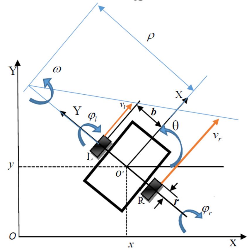
importance, since virtually every task requires the robot to II. MODELING OF A MOBILE ROBOT
travel between different positions by tracking a desired The differential mobile robot is a platform with two
trajectory while being able to localize itself and plan its future motorized wheels (Figure 1), mounted on the same axis and
movements without human assistance [4] in order to controlled independently while having in addition a free front
accomplish the defined task [5]. Therefore, once the trajectory
Corresponding author: Boucetta Kasmi
www.etasr.com Kasmi & Hassam: Comparative Study between Fuzzy Logic and Interval Type-2 Fuzzy Logic …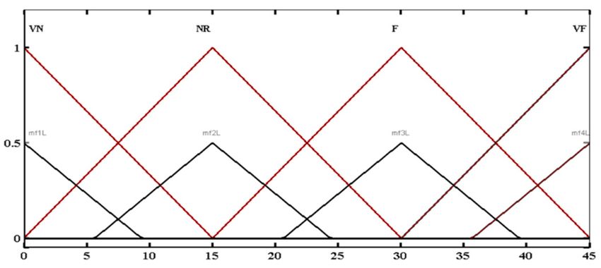
Engineering, Technology & Applied Science Research Vol. 11, No. 2, 2021, 7011-7017 7012
wheel [7]. The simplified hypotheses considered for modeling r r
are: v 2 2 ϕ& r
• The ground wheel contact is a contact point. ω = r
r ϕ&
(3)
− l
• The rolling of each wheel is done without slipping. 2b 2b
The generalized coordinates of the system are given by where v and ω are respectively the linear and angular velocities
q = [ x , y , θ , ϕ r , ϕ l ]T where [x, y] are the Cartesian of the mobile robot and 2b and r represent respectively the
radius of the wheels and the distance between them.
coordinates of the mobile robot, θ is its orientation measured
from the x-axis and ϕ r , ϕl are the angular positions of the right The non-holonomic constraint is represented in a simple
and left wheel respectively [2, 3]. mathematical form [3]:
x& cos(θ ) − y& sin(θ ) = 0 (4)
Equation (4) implies that a perfect tracking is achievable
only if the reference trajectories are feasible for the physical
platform.
IV. LOCALIZATION OF A MOBILE ROBOT
One of the fundamental problems of autonomous mobile
robotics is the locationing of the robot during its movement. In
fact, to locate a mobile robot is to determine, in a given work
reference, its position and its orientation, in order to
accomplish the control structure that is based on these data.
A. Presentation of the Odometry
The odometry allows determining the position and the
orientation of a mobile robot navigating on a plane ground,
with respect to the reference mark, which is the robot’s mark in
its initial configuration. This technique is based on the
integration of the elementary motions of the wheels measured
by means of incremental encoders.
Fig. 1. The unicycle-type mobile robot under study. B. The Odometry for the Localization of a Mobile Robot
This locomotion system is very popular for indoor robots
III. KINEMATIC MODEL OF THE MOBILE ROBOT because of its maneuverability and ease of operation. In this
The kinematic model of the mobile robot can be written as case, the displacement ∆D and the elementary rotation ∆θ of
[3]: the robot model in the plane can be expressed as a function of
the elementary displacements of the right and left wheels
r cos(θ ) r cos(θ ) respectively ∆d r and ∆dl , by [13, 14]:
2
x& 2
y& r sin(θ ) r sin(θ ) ∆d r + ∆d l
∆D = (5)
2 2 ϕ&r 2
q& = θ& = = (1)
r − r ϕ&l ∆d r − ∆d l
ϕ&r 2b ∆θ = (6)
2b 2b
ϕ&
l 1 0
where ( xk , yk ,θ k ) is the configuration of the robot at the
0 1 instant k, and ( ∆Dk , ∆θ k ) the components of the elementary
By introducing the following control inputs: displacement measured between instants k and k+1. The
elementary rotation at time k+1 is:
ϕ& r b 1 1 v
& = θ k +1 = θ k + ∆θ k (7)
ϕl r 1 −1 ω
These very simple formulas are obtained by considering
Equation (1) may be written as:
that the robot moves in a straight line ∆Dk in the direction
x& cos(θ ) 0 defined by θ k , and then makes a rotation on site of ∆θk :
y& = sin(θ ) v + 0 ω (2) ∆θ k
θ& 0 xk +1 = xk + ∆Dk cos(θ k + ) (8)
1 2
www.etasr.com Kasmi & Hassam: Comparative Study between Fuzzy Logic and Interval Type-2 Fuzzy Logic …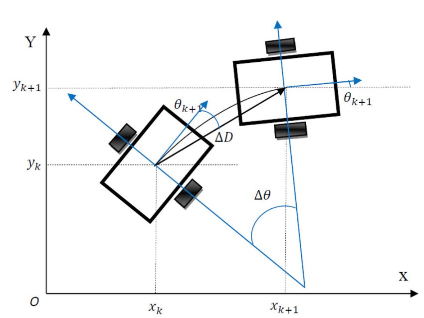
Engineering, Technology & Applied Science Research Vol. 11, No. 2, 2021, 7011-7017 7013
∆θ k
y k +1 = yk + ∆Dk sin(θ k + ) (9)
2
This robot control was applied in both FL and IT-2FL
strategies.
Fig. 4. Structure of the proposed navigation system.
Fig. 5. The mobile robot in a free environment.
Fig. 2. The odometry applied to the mobile robot. 1) Input Variables
For the robot-target distance d (m), we have chosen 4
V. S TRUCTURE OF THE FL CONTROLLER membership functions (Figure 6): very near (VN), near (NR),
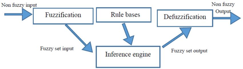
A classic fuzzy controller consists of a fuzzification far (F), and very far (VF) distributed over the discourse
interface, a rule base, an inference system, and a universe [0, 30]. For the entry θ (rad), the robot-target angle
defuzzification interface [15-21]. The structure of an FL system has 7 membership functions that are associated (Figure 7):
is illustrated in Figure 3. negative big (NB), negative medium (NM), negative small
(NS), zero (Z), positive small (PS), positive medium (PM), and
positive big (PB) distributed over the discourse universe [-3, 3].
Fig. 3. Structure of an FL system.
In our work, the fuzzy controller (FL and IT-2FL) has 4
triangular-shaped membership functions for the robot-target
distance, 7 membership functions for the variation of the robot-
target angle and an interval-type of fuzzy sets for the linear
velocity and angular velocity output for IT-2FLC. The output Fig. 6. The membership functions of the input variable distance d.
variables for FLC are 4 triangular-shaped membership
functions for linear velocity and 7 triangular-shaped
membership functions for the angular velocity.
VI. THE PROPOSED NAVIGATION SYSTEM
The movement of the unicycle robot is carried out on a flat
ground and the position of the robot can be expressed at every
moment according to its kinematic model (x, y, θ ). When
meeting obstacles or walls, the relevant decision is made by
two controllers. Figure 4 shows the structure of the system,
consisting of a free navigation controller and an obstacle
avoidance controller [8-10]. Fig. 7. The membership functions of the input variable θ.
A. Implementation of the Free Navigation Controller 2) Output Variables
If we take a mobile robot operating in a non-binding For the linear velocity v (m/s), 4 intervals were chosen:
environment, then the optimal path from an initial very slow (VS), slow (S), fast (F), and very fast (VF)
configuration to a final situation would naturally be a straight distributed over the discourse universe [0, 0.2].
line joining the two situations (Figure 5) [8, 11, 12].
www.etasr.com Kasmi & Hassam: Comparative Study between Fuzzy Logic and Interval Type-2 Fuzzy Logic …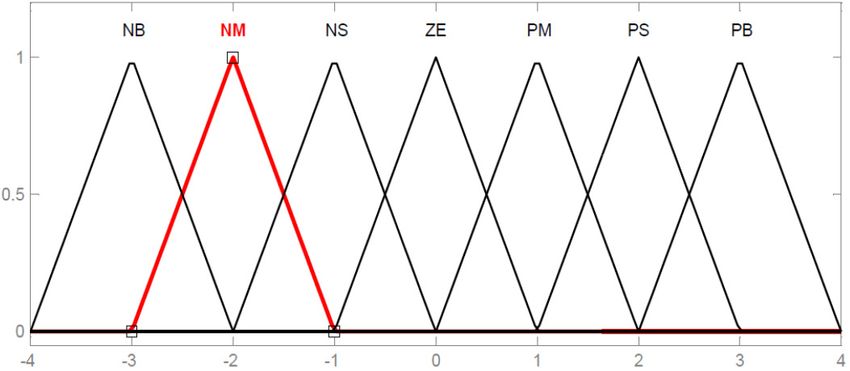
Engineering, Technology & Applied Science Research Vol. 11, No. 2, 2021, 7011-7017 7014
The angular velocity ω (rad) has seven (7) intervals: Rule 28: IF d is VF AND θ is PB
negative big (NB), negative medium (NM), negative small
(NS), zero (Z), positive small (PS), positive medium (PM) and THEN v is S AND ω is NM
positive big (PB), distributed over the discourse universe [-0.8, We applied these rules of the free navigation controller in
0.8]. both FL and IT-2FL strategies.
3) Representation of Input Variables B. Implementation of the Obstacle Avoidance Controller
The membership functions of the triangular input variables In the case where the robot moves close to an obstacle,
are shown in Figures 8, 9. another fuzzy controller is used to avoid the obstacle and steer
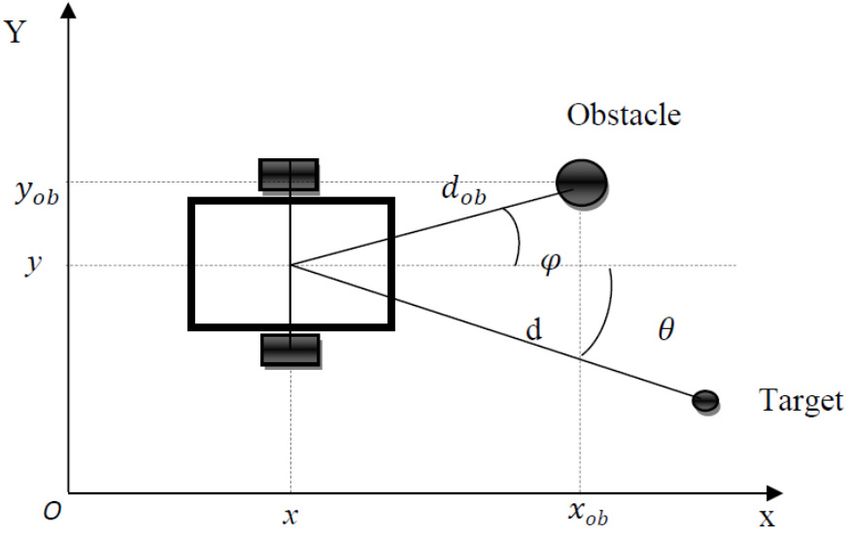
the robot away from d ob using the navigation controller. Figure
10 shows the configuration of the robot in the obstacle area [12,
14, 20].
Fig. 8. The membership functions of the input variable d in Matlab
Toolbox.
Fig. 10. The mobile robot in an environment with an obstacle.
The obstacle avoidance controller that we used has two
input variables: robot-obstacle distance and robot-obstacle
angle ( d ob and φ) respectively and two output variables: robot
linear velocity v and angular velocity ω.
1) The Membership Functions of the Input Variables for FLC
Fig. 9. The membership functions of the input variable θ in Matlab
Toolbox.
4) The Rule of the Free Navigation Controller
TABLE I. THE RULE BASE OF THE FREE NAVIGATION CONTROLLER
Distance d
Orientation θ
VN N F VF
NB VS, PB VS, PB S, PB S, PM
NM VS, PM VS, PS S, PS F, PS
NS VS, S S, PS F, PS F,PS
Z VS, Z S, Z F, Z V, FZ Fig. 11. The membership functions of the input variable dob.
PS VS, NS S, NS F, NS VF, NS
PM VS, NM VS, NM F, NM F, NS
PB VS, NB VS, NB S, NB S, NB
The rule base of the free navigation controller is the
following:
Rule 1: IF d is VN AND θ is NB
THEN v is VS AND ω is PB
Rule 2: IF d is VN AND θ is NM
THEN v is VS AND ω is PM
………………………………………………. Fig. 12. The membership functions of the input variable φ.
www.etasr.com Kasmi & Hassam: Comparative Study between Fuzzy Logic and Interval Type-2 Fuzzy Logic …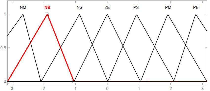
Engineering, Technology & Applied Science Research                 Vol. 11, No. 2, 2021, 7011-7017                                                               7015

2) The Membership Functions of the Input Variables for IT-                                                              VII. S IMULATION RESULTS
2FLC                                                                       To compare the control and planning performances of FL
                                                                        and IT2-FL controllers, simulations were conducted and
                                                                        analyzed with MATLAB Fuzzy Logic Toolbox R2014a.
                                                                        A. Trajectory without Obstacles
                                                                              From Figure 15, we notice that from its initial position,
                                                                        ( x i =2.5 and yi =4.5, θ =45°) the mobile robot could reach the
                                                                        target whose coordinates are (xf =7, yf =−1). In Figures 16 and
                                                                        17 we can see the velocity and the angular velocity of the
                                                                        mobile robot. From the obtained results, we notice that the
                                                                        mobile robot adopts the following behavior: when the robot-
Fig. 13. The membership functions of the input variable dob in Matlab   target angle is large, the angular velocity is high, whereas the
Toolbox.                                                                linear velocity is small. Once the robot-target angle becomes
                                                                        zero, the linear velocity reaches its maximum. The latter
                                                                        gradually decreases by canceling once the target is reached.

                                                                                                           8

                                                                                                           7

                                                                                                           6

                                                                                                           5

                                                                                                           4

                                                                                                           3
                                                                                                   Y( m)

                                                                                                                                                           IT2-FLC
                                                                                                           2
Fig. 14. The membership functions of the input variable φ in Matlab
                                                                                                           1
Toolbox.                                                                                                                                         FLC
                                                                                                           0

3) The Rule Base of the Obstacle avoidance controller                                                  -1

                                                                                                       -2
         TABLE II.     THE RULE BASE OF THE OBSTACLE AVOIDANCE                                          -2                   0         2               4          6            8
                                CONTROLLER                                                                                                  X( m)

                               The obstacle distance dob                                  Fig. 15.                    Attraction to the target: barrier-free environment.
      Orientation φ
                         VN            N            F      VF
          NB            VS, PM      VS, PM       S, PM   S, PM                                     0. 06
          NM            VS, PM       VS, PS      S, PS    F, PS                                                                                                       F LC
          NS            VS, PS       S, PS       F, PS    F,PS                                    0 .0 55
                                                                                                                                                                      IT 2 -F LC

           Z            VS, PM       S, NS       F, PS   VF, PS
          PS            VS, NM       S, NS       F, NS   VF, NS                                    0. 05

          PM            VS, NM      VS, NM       F, NS    F, NS
                                                                              The velocity(m/s)

                                                                                                  0 .0 45
          PB            VS, NB      VS, NB       S, NB   S, NB
                                                                                                   0. 04
    The rule base of the obstacle avoidance controller is the
following:                                                                                        0 .0 35

   Rule 1: IF d ob is VN AND ϕ is NB                                                               0. 03

           THEN v is VS AND         ω   is PM                                                     0 .0 25

   Rule 2: IF d ob is VN AND ϕ is NM                                                               0. 02
                                                                                                               0       100       200       300      400    5 00       6 00         7 00
                                                                                                                                             Time(s)

           THEN v is VS AND         ω   is PM                                                                      Fig. 16.      The velocity of the mobile robot.

   ……………………………………………….                                                  B. Obstacle Avoidance
   Rule 28: IF d ob is VF AND ϕ is PB                                      From Figure 18 we can see how the mobile robot reached
                                                                        the target (xf =6, yf =7) from its initial position ( x i =3 and
           THEN v is S AND        ω   is NB
                                                                        yi =8, θ =−45°).
    We applied these rules of the obstacle avoidance controller
in both the FL and IT-2FL strategies.

       www.etasr.com                          Kasmi & Hassam: Comparative Study between Fuzzy Logic and Interval Type-2 Fuzzy Logic …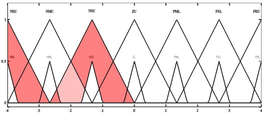
Engineering, Technology & Applied Science Research Vol. 11, No. 2, 2021, 7011-7017 7016
have designed the FL and IT-2FL controllers and simulated the
1.5
FLC mobile robot movement from an initial to a desired position in
IT -2FLC different environment configurations, with and without
1
obstacles. The proposed fuzzy control exploits the interactive
The angular velcity (rad/s)
variables between the mobile robot and the unknown
0.5
environment to generate the robot’s velocity and steering,
which makes it possible to bring the mobile robot towards the
0
target while avoiding any obstacles present in this environment.
-0.5
1.5
-1 1
FLC
0.5 IT2-FLC
-1.5
0 100 200 3 00 40 0 500 600 700
The velocity (m/s)
Time(s)
0
Fig. 17. The angular velocity of the mobile robot.
-0.5
10
-1
9
-1.5
8
-2
0 100 200 300 400 500
Y(m)
Time (s)
7
Fig. 20. The velocity of the mobile robot in the presence of obstacles.
6
0. 8
5 FLC
0. 6 IT 2-FLC
4
0 1 2 3 4 5 6 7 8
The angular velocity (rad/s)
0. 4
X(m)
Fig. 18. Convergence towards the target by FLC in the presence of 0. 2
obstacles.
0
10
- 0.2
9 - 0.4
- 0.6
8
- 0.8
0 100 200 300 400 500
Y(m)
7 Time(s)
Fig. 21. The angular velocity of the mobile robot in the presence of
6 obstacles.
5 In order to test the applicability of the IT-2FLC system, we
compared its performance with that of an FL controller. The
4
0 1 2 3 4 5 6 7 8
IT-2FLC offers better results than its FL counterpart in
X(m) environments with obstacles. The main characteristic of the IT-
Fig. 19. Convergence towards the target by IT-2FLC in the presence of
2FLC sets is its ability to handle uncertainties more efficiently
obstacles. than FLC. This is made possible because a larger number of
parameters and more freedom degrees are available in the IT-
We can highlight from the above results that the IT-2FL 2FLC sets.
sets can be quite useful when considering the control of a
mobile robot. It was shown in depth that the proposed IT2-FL REFERENCES
controller is more efficient in terms of saving time, smooth [1] P. Gil, Y. Mezouar, M. Vincze, and J. A. Corrales, "Robotic Perception
trajectory, and optimal distance than its FL counterpart. of the Sight and Touch to Interact with Environments," Journal of
Sensors, vol. 2016, Dec. 2016, Art. no. e1751205, https://doi.org/
VIII. CONCLUSION 10.1155/2016/1751205.
[2] U. Libal and J. Płaskonka, "Noise sensitivity of selected kinematic path
In this paper, movement control methods of a wheeled following controllers for a unicycle," Bulletin of the Polish Academy of
mobile robot were studied. To achieve this control target, we Sciences, Technical Sciences, vol. 62, no. 1, pp. 3–13, Mar. 2014,
https://doi.org/10.2478/bpasts-2014-0001.
www.etasr.com Kasmi & Hassam: Comparative Study between Fuzzy Logic and Interval Type-2 Fuzzy Logic …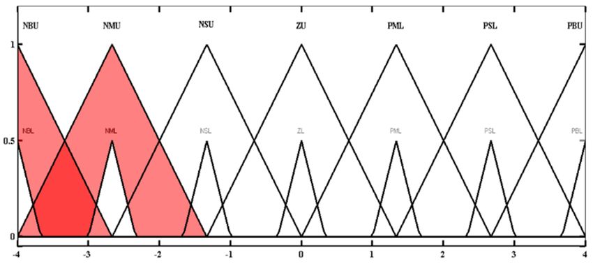
Engineering, Technology & Applied Science Research                          Vol. 11, No. 2, 2021, 7011-7017                            7017
[3]    G. Abdelhakim and H. Abdelouahab, "A New Approach for Controlling           [21] H. A. Hagras, "A hierarchical type-2 fuzzy logic control architecture for
       a Trajectory Tracking Using Intelligent Methods," Journal of Electrical          autonomous mobile robots," IEEE Transactions on Fuzzy Systems, vol.
       Engineering & Technology, vol. 14, no. 3, pp. 1347–1356, May 2019,               12, no. 4, pp. 524–539, Aug. 2004, https://doi.org/10.1109/TFUZZ.
       https://doi.org/10.1007/s42835-019-00112-1.                                      2004.832538.
[4]    B. Hua, E. Rama, G. Capi, and M. Jindai, "A human-like robot
       intelligent navigation in narrow indoor environments," International
       Journal of Information and Electronics Engineering, vol. 6, no. 5, pp.
       308–312, Sep. 2016, https://doi.org/10.18178/IJIEE.2016.6.5.644.
[5]    K. Chen, F. Yang, and X. Chen, "Planning with task-oriented knowledge
       acquisition for a service robot," in Proceedings of the Twenty-Fifth
       International Joint Conference on Artificial Intelligence, New York, NY,
       USA, Jul. 2016, pp. 812–818.
[6]    Y. Gigras and K. Gupta, "Artificial Intelligence in Robot Path Planning,"
       International Journal of Soft Computing and Engineering, vol. 2, no. 2,
       pp. 471–474, May 2012.
[7]    B. Damas and J. Santos-Victor, "Avoiding moving obstacles: the
       forbidden velocity map," in 2009 IEEE/RSJ International Conference on
       Intelligent Robots and Systems, St. Louis, MO, USA, Oct. 2009, pp.
       4393–4398, https://doi.org/10.1109/IROS.2009.5354210.
[8]    W. Yu, J. Peng, X. Zhang, and K.-C. Lin, "A Cooperative Path Planning
       Algorithm for a Multiple Mobile Robot System in a Dynamic
       Environment," International Journal of Advanced Robotic Systems, vol.
       11, no. 8, Aug. 2014, Art. no. 136, https://doi.org/10.5772/58832.
[9]    Xiaoyu Yang, M. Moallem, and R. V. Patel, "A layered goal-oriented
       fuzzy motion planning strategy for mobile robot navigation," IEEE
       Transactions on Systems, Man, and Cybernetics, Part B (Cybernetics),
       vol. 35, no. 6, pp. 1214–1224, Dec. 2005, https://doi.org/10.1109/
       TSMCB.2005.850177.
[10]   D. J. Huh, J. H. Park, U. Y. Huh, and H. I. Kim, "Path planning and
       navigation for autonomous mobile robot," in IEEE 2002 28th Annual
       Conference of the Industrial Electronics Society. IECON 02, Seville,
       Spain, Nov. 2002, vol. 2, pp. 1538–1542, https://doi.org/10.1109/
       IECON.2002.1185508.
[11]   J. Courbon, Y. Mezouar, L. Eck, and P. Martinet, "A generic framework
       for topological navigation of urban vehicle," presented at the ICRA09 -
       Workshop on Safe navigation in open and dynamic environments
       Application to autonomous vehicles, May 2009.
[12]   T. Belker and D. Schulz, "Local action planning for mobile robot
       collision avoidance," in IEEE/RSJ International Conference on
       Intelligent Robots and Systems, Lausanne, Switzerland, Sep. 2002, vol.
       1, pp. 601–606, https://doi.org/10.1109/IRDS.2002.1041457.
[13]   M. Defoort, J. Palos, A. Kokosy, T. Floquet, W. Perruquetti, and D.
       Boulinguez, "Experimental Motion Planning and Control for an
       Autonomous Nonholonomic Mobile Robot," in Proceedings 2007 IEEE
       International Conference on Robotics and Automation, Rome, Italy,
       Apr.     2007,     pp.   2221–2226,       https://doi.org/10.1109/ROBOT.
       2007.363650.
[14]   E.-H. Guechi, J. Lauber, and M. Dambrine, "Suivi de trajectoire d’un
       robot mobile non holonome en présence de retards sur les mesures," in
       2010 IEEE CIFA, Nancy, France, 2010.
[15]   N. N. Karnik, J. M. Mendel, and Qilian Liang, "Type-2 fuzzy logic
       systems," IEEE Transactions on Fuzzy Systems, vol. 7, no. 6, pp. 643–
       658, Dec. 1999, https://doi.org/10.1109/91.811231.
[16]   O. Kahouli, B. Ashammari, K. Sebaa, M. Djebali, and H. H. Abdallah,
       "Type-2 Fuzzy Logic Controller Based PSS for Large Scale Power
       Systems Stability," Engineering, Technology & Applied Science
       Research, vol. 8, no. 5, pp. 3380–3386, Oct. 2018, https://doi.org/
       10.48084/etasr.2234.
[17]   O. Castillo and P. Melin, Type-2 Fuzzy Logic: Theory and Applications.
       Berlin Heidelberg, Germany: Springer-Verlag, 2008.
[18]   B. Bouchon-Meunier and C. Marsala, Logique floue. Principes, aide à la
       décision. Paris, France: Hermes Science Publications, 2002.
[19]   Qilian Liang and J. M. Mendel, "Interval type-2 fuzzy logic systems:
       theory and design," IEEE Transactions on Fuzzy Systems, vol. 8, no. 5,
       pp. 535–550, Oct. 2000, https://doi.org/10.1109/91.873577.
[20]   N. N. Karnik and J. M. Mendel, "Type-2 fuzzy logic systems: type-
       reduction," in SMC’98 Conference Proceedings. 1998 IEEE
       International Conference on Systems, Man, and Cybernetics, San Diego,
       CA, USA, Oct. 1998, vol. 2, pp. 2046–2051, https://doi.org/
       10.1109/ICSMC.1998.728199.

          www.etasr.com                              Kasmi & Hassam: Comparative Study between Fuzzy Logic and Interval Type-2 Fuzzy Logic …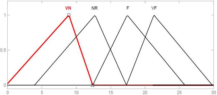
You can also read