Spike Train Coactivity Encodes Learned Natural Stimulus Invariances in Songbird Auditory Cortex
←
→
Page content transcription
If your browser does not render page correctly, please read the page content below
The Journal of Neuroscience, January 6, 2021 • 41(1):73–88 • 73

Systems/Circuits

Spike Train Coactivity Encodes Learned Natural Stimulus
Invariances in Songbird Auditory Cortex
Brad Theilman,1 Krista Perks,1 and Timothy Q. Gentner1,2,3,4
1
 Neurosciences Graduate Program, University of California San Diego, La Jolla, California 92093, 2Department of Psychology, University of
California San Diego, La Jolla, California 92093, 3Neurobiology Section, Division of Biological Sciences, University of California San Diego, La Jolla,
California 92093, and 4Kavli Institute for Brain and Mind, La Jolla, California 92093

The capacity for sensory systems to encode relevant information that is invariant to many stimulus changes is central to nor-
mal, real-world, cognitive function. This invariance is thought to be reflected in the complex spatiotemporal activity patterns
of neural populations, but our understanding of population-level representational invariance remains coarse. Applied topology
is a promising tool to discover invariant structure in large datasets. Here, we use topological techniques to characterize and
compare the spatiotemporal pattern of coactive spiking within populations of simultaneously recorded neurons in the second-
ary auditory region caudal medial neostriatum of European starlings (Sturnus vulgaris). We show that the pattern of popula-
tion spike train coactivity carries stimulus-specific structure that is not reducible to that of individual neurons. We then
introduce a topology-based similarity measure for population coactivity that is sensitive to invariant stimulus structure and
show that this measure captures invariant neural representations tied to the learned relationships between natural vocaliza-
tions. This demonstrates one mechanism whereby emergent stimulus properties can be encoded in population activity, and
shows the potential of applied topology for understanding invariant representations in neural populations.
Key words: auditory; invariance; population; topology

     Significance Statement
     Information in neural populations is carried by the temporal patterns of spikes. We applied novel mathematical tools from
     the field of algebraic topology to quantify the structure of these temporal patterns. We found that, in a secondary auditory
     region of a songbird, these patterns reflected invariant information about a learned stimulus relationship. These results dem-
     onstrate that topology provides a novel approach for characterizing neural responses that is sensitive to invariant relation-
     ships that are critical for the perception of natural stimuli.

Introduction                                                                                                       nature of this coordination and how it supports invariance is an
Functional sensory systems must express a degree of representa-                                                    important open question in neuroscience.
tional invariance to convey relationships or abstract properties,                                                       Most current methods for quantifying neuronal population
such as category membership, between otherwise distinguishable                                                     structure rely on converting spiking activity into a vector of in-
stimuli. At the neural level, invariant representations may mani-                                                  stantaneous firing rates (Cunningham et al., 2009; Churchland et
fest as robustness to “noise,” or consistency across trials or                                                     al., 2012; Gallego et al., 2018). Over time, these vectors trace out
learned stimuli in a single animal, or across animals. For high-                                                   a path in a high-dimensional space. The dynamics of this path
dimensional natural signals in particular, whose representation is                                                 can be correlated with simultaneous information about the stim-
distributed, invariant representations likely involve the coordi-                                                  ulus or behavior. However, these methods require averaging
nated spiking activity of neuronal populations across time. The                                                    activity over time or space to overcome putative noise in single-
                                                                                                                   neuron firing rates. This is problematic for populations that
                                                                                                                   must represent intrinsically time-varying objects, such as vocal
Received Jan. 31, 2020; revised Oct. 30, 2020; accepted Oct. 31, 2020.                                             communication signals, on fast time scales. Auditory populations
   Author contributions: B.T., K.P., and T.Q.G. designed research; B.T. and K.P. performed research; B.T.
analyzed data; B.T. wrote the first draft of the paper; B.T., K.P., and T.Q.G. edited the paper; B.T. and T.Q.G.
                                                                                                                   that do so often exhibit lifetime-sparse firing, sometimes compli-
wrote the paper.                                                                                                   cating the estimation of instantaneous firing rates. Thus, while
   This work was supported by National Institutes of Health DC0164081 and DC018055 to T.Q.G. We thank              firing rate vectors may be decodable in some cases (Ince et al.,
Charles Stevens for comments on an earlier draft.                                                                  2013; Rigotti et al., 2013), they belie the near instantaneous and
   The authors declare no competing financial interests.
   Correspondence should be addressed to Timothy Q. Gentner at tgentner@ucsd.edu.
                                                                                                                   continuous nature of natural perception.
   https://doi.org/10.1523/JNEUROSCI.0248-20.2020                                                                       Alternatively, information may be carried in patterns of coin-
Copyright © 2021 the authors                                                                                       cident spiking, or a “coactivation code” (Curto and Itskov, 2008;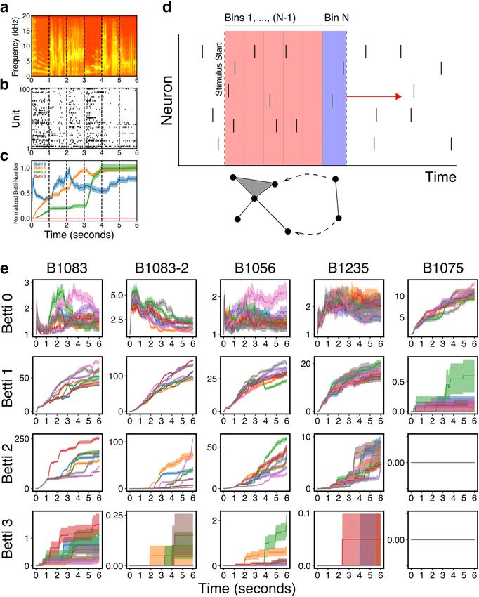
74 • J. Neurosci., January 6, 2021 • 41(1):73–88                                                               Theilman et al. · Topology of Auditory Representation

Brette, 2012). Curto and Itskov (2008) developed an algorithm                     Stimuli. Starlings (both male and female) produce long, spectrotem-
for converting neural coactivity into a kind of topological space             porally rich, and individualized songs composed of repeating, shorter
called a simplicial complex. The spatial structure of this complex            acoustic segments known as “motifs” that are learned over the bird’s life-
is determined by the relative timing of spikes in a population.               span. Motifs are on the order of 0.5–1.5 s in duration. In these experi-
                                                                              ments, a library of 16 6-s-long “pseudo-songs” were used as stimuli.
Their simulations showed that invariant topological measures of
                                                                              Each pseudo-song was constructed from six 1-s-long motifs manually
the spike-derived simplicial complex matched several measures                 extracted from a larger library of natural starling song produced by sev-
of the space of stimuli driving the neural response. This powerful            eral singers. The first motif of each pseudo-song was an introductory
property allowed them to reconstruct some stimulus space prop-                whistle motif, as commonly occurs in natural starling songs. The same
erties solely from the population activity without having to corre-           whistle was used for all 16 pseudo-songs. After the introductory whistle,
late physical positions to population firing rates (i.e., compute             all motifs were unique to one pseudo-song (i.e., none of the other motifs
receptive fields). To our knowledge, this topological approach                occurred in more than one song). The amplitude of each pseudo-song
has not been used to examine the invariant properties of the tem-             was normalized to 65 dB SPL.
poral coactivation patterns of in vivo sensory system responses.                  Behavioral training. We trained 4 birds on a two-alternative forced-
    Here, we apply the Curto-Itskov construction to extracellular             choice task to recognize four naturalistic pseudo-song stimuli, following
                                                                              previously described operant conditioning procedures (Knudsen and
responses from the caudal medial neostriatum (NCM), a second-
                                                                              Gentner, 2013). Briefly, the operant apparatus afforded access to three
ary auditory cortical region, in European starlings, a species of             separate response ports. Subjects learned to peck at the center response
songbird. Starlings adeptly learn complex acoustic signals and                port to trigger the playback of one of four pseudo-songs associated with
provide an important model for the neural basis of vocal learning             two different responses: a peck to the left response port or a peck to the
and perception (Kiggins et al., 2012). The NCM, an auditory                   right response port. Pecking at the left response port following the pre-
forebrain region analogous to secondary auditory cortex in                    sentation of two songs, or at the right response port following the other
mammals (Karten, 1967; Vates et al., 1996; Wang et al., 2010), is             two songs, allowed for brief (1–2 s) access to a food hopper. Incorrect
involved in processing complex behaviorally relevant acoustic                 responses, pecking the response port not associated with a given song,
signals (birdsongs) (Sen et al., 2001; Grace et al., 2003; Thompson           resulted in a short timeout during which the house light was extin-
                                                                              guished and the bird could not feed from the hopper. The 12 remaining
and Gentner, 2010). NCM neurons respond selectively to subsets
                                                                              pseudo-songs were never presented during operant training for that
of conspecific songs (Bailey et al., 2002; De Groof et al., 2013),            bird. Assignment of songs for behavioral training was counterbalanced
and single-neuron responses display complex receptive fields                  across subjects. The accuracy of the birds over the last 500 trials before
(Theunissen et al., 2000; Kozlov and Gentner, 2016). How the                  neural recording was as follows: B1083, 86.2%; B1056, 95.4%; B1235,
responses of single NCM neurons combine to represent invari-                  97.6%; B1075, 91.2%. All birds exceeded 90% accuracy during training.
ant structure from natural vocal signals at the population level              Acquisition of the behavior was fast; the number of 500 trial blocks
remains unknown. We hypothesized that invariant song repre-                   required to first exceed 90% accuracy was as follows: B1083, 30; B1056,
sentations in NCM are carried in the coactivation pattern of                  14; B1235, 5; B1075, 13.
spikes in the population, and that these patterns manifest as a                   Electrophysiology. Once trained, we prepared the birds for physiolog-
                                                                              ical extracellular recording from caudo-medial nidopallium (NCM). We
topologically invariant structure. Our results support this hy-
                                                                              anesthetized birds (20% urethane, 7 ml/kg, i.m.), affixed a metal pin to
pothesis. We show that the coactivity-based topology of NCM                   their skull with dental cement, removed an ;1 mm2 window from the
neural activity is nontrivial and carries stimulus-specific infor-            top layer of skull, and placed a small craniotomy dorsal to NCM. We
mation. Using a novel mathematical approach to compare sim-                   inserted a 16- or 32-channel silicon microelectrode (NeuroNexus
plicial complexes, we find evidence that temporal coactivity                  Technologies) through the craniotomy into the NCM of the head-fixed
patterns in NCM represent both stimulus identity and learned                  bird positioned on a foam couch within a sound attenuation chamber
relationships between stimuli. We suggest that understanding                  (Acoustic Systems). Auditory stimuli were presented from a speaker
the topology of sensory-driven neural population coactivity                   mounted ;20 cm above the center of the bird’s head, at a mean level of
offers novel insight into the nature of how invariant representa-             60 dB SPL measured at 20 cm. The microelectrode was lowered until all
tions are constructed from complex natural signals by neural                  recording sites were within NCM, and then allowed to sit for ;15 min
                                                                              to allow any tissue compression that might have occurred during inser-
populations.
                                                                              tion to relax and stabilize before stimulus presentations began. Auditory
                                                                              activity was confirmed by exposing the birds to non–task-related sounds
Materials and Methods                                                         and observing sound-evoked responses in the raw voltage signal on one
                                                                              or more channels. The 16 pseudo-song stimuli in the block were pre-
Experimental model and subject details                                        sented pseudo-randomly until a total of 20 repetitions for each stimulus.
All protocols were approved by the University of California San Diego         For B1083, after the completion of the first block, the electrode was
Institutional Animal Care and Use Committee. This study did not gener-        driven deeper into NCM by a distance greater than the electrode length,
ate new unique reagents. All of the custom code used for the topological      to obtain another block from a disjoint population. Raw voltages recorded
analyses described here is available at https://github.com/theilmbh/          from each microelectrode site were buffered and amplified (20 gain)
NeuralTDA. Requests for resources, reagents, and further information is       through a headstage (TBSI), bandpass filtered between 300 Hz and 5 kHz,
available from T.Q.G.                                                         and amplified (AM Systems, model 3600) and sampled digitally at 20 kHz
    Subjects. Four birds were used in the study, identified as B1083,         (16 bit; CED model 1401) via Spike2 software (CED). We saved the full
B1056, B1235, and B1075. All birds were wild-caught in southern               waveforms for offline analysis.
California and housed communally in large flight aviaries before training
and physiological testing. During behavioral training, birds were housed      Experimental design and statistical analysis
in isolation along with a custom operant apparatus in sound-attenuation           Spike sorting. Extracellular waveforms were spike-sorted offline using
chambers (Acoustic Systems) and maintained on a light schedule that           the Phy spike sorting framework (Rossant et al., 2016). After automatic
followed local sunrise and sunset times. Birds had unrestricted access to     clustering, the sort was completed manually using the KwikGUI inter-
water at all times. During behavioral training, birds received all food       face. Clusters with large signal-to-noise ratio and ,1% refractory period
(chick chow) through the operant apparatus, contingent on task per-           violations (taken to be 1 ms) were labeled as “Good” clusters and
formance. All subjects were at least 1 year of age or older at the start of   included in the analysis. Because the analyses are meant to quantify pop-
the experiment. We did not control for the sex of the subjects.               ulation-level structure, sorting priority was given to extracting as many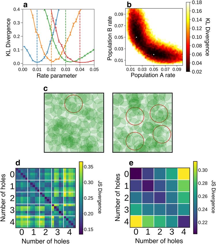
Theilman et al. · Topology of Auditory Representation                                                                J. Neurosci., January 6, 2021 • 41(1):73–88 • 75

neural signals as possible. Clusters identified automatically were mostly      is a spike count in the time window dt. The spike counts were then di-
kept separate unless obvious duplicates were observed. Duplicate clusters      vided by the window width to determine a “firing rate” for that cell in
were defined by overlapping distributions in PCA space, similar wave-          that time bin. The time average was taken to yield an N_cells  N_trials
form shape, and cross-correlations that respected refractory periods.          matrix of average instantaneous firing rates for each cell for each trial.
Despite these measures, the set of clusters labeled “Good” are likely to       Then, the multidimensional array D was thresholded by determining
contain multiunit activity as well as single units.                            which bins had a firing rate greater than some threshold value times the
     Data processing. Data processing began by converting the neural           average firing rate. This yielded an N_cells  N_bins  N_trials binary
population activity on each trial into an n  m matrix comprising all the      array B that represents significantly active cells. Unless otherwise noted,
spikes across all the isolated clusters and binned into 10 ms windows          the threshold value of 4 times the average firing rate of the unit was
with a 5 ms overlap between windows. We used the Perseus persistent            used. Since the average firing rate of the units was low, the threshold
homology software for computing Betti numbers from simplicial com-             value did not make a significant impact on the results.
plexes (Mischaikow and Nanda, 2013). For computing samples from the                For each trial and for each time bin in B, the N_cell-long binary vec-
simplicial configuration model, we used the code described by Young et         tor V was used to create a list of cells that were active in that time bin.
al. (2017). All other computations were performed using custom-written         This was repeated across all time bins to create a list of “cell groups”
Python and C code available at http://github.com/theilmbh/NeuralTDA.           active during the trial, much like the cell groups defined by Curto and
     Mathematical background. Outside of neuroscience, invariance has          Itskov (2008). This list of cell groups was taken to define the maximal
been the subject of intense mathematical investigation. In particular, the     simplexes for the simplicial complex. Using algorithms derived from
mathematical field of topology is dedicated to studying the properties of      published work (Kaczynski et al., 2006), this list of cell groups was
arbitrary spaces that are invariant to different classes of transformations.   turned into a list of lists of basis vectors for the chain complex. The n-th
This research has produced a wealth of techniques and methods for              sublist represents the chain complex basis vectors corresponding to the n-
defining and quantifying invariant structures. Recently, these techniques      dimensional simplexes in the simplicial complex. We also computed the
have been increasingly applied to the problem of finding invariant struc-      matrices that represent the boundary operators in the chain complex.
ture in large datasets. Topology takes a global viewpoint, and the “quan-          Betti curves. Homology is one of the most basic topological invari-
tities” of interest are entire spaces, rather than single numerical            ants one can use to describe a topological space. Loosely speaking,
measures. By converting neural population activity into a topological          homology counts the number of n-dimensional holes in the space. These
space instead of reducing it to a series of numerical measures, we gain        holes are described purely algebraically by computing how n-dimen-
access to the library of techniques topology offers for characterizing         sional cycles (e.g., a circle) are not the boundary of an n 1 1-dimensional
invariant structure.                                                           simplex. For each dimension n, the number of such holes is called the n-
     Here, we introduce the basics of the mathematics used for our analy-      th Betti number. The reason that Betti numbers are a useful characteriza-
sis. More thorough introductions are available elsewhere (Hatcher,             tion of the topological spaces we construct is that any two topological
2002), including for the many applications of algebraic topology (Ghrist,      spaces that differ in their Betti numbers cannot be topologically equiva-
2014). Our analyses work by constructing mathematical objects known            lent. Furthermore, topological holes interpreted neurally represent
as simplicial complexes. Simplicial complexes are topological spaces that      “gaps” in the coactivation pattern (which neurons do not fire together)
are built from discrete building blocks known as simplexes. For each           and thus carry information about how the population activity is struc-
dimension, there is only one prototype simplex. For example, 0-dimen-          tured. We summarized the topology of neurally derived simplicial com-
sional simplexes are points, 1-dimensional simplexes are line segments,        plexes by computing these Betti numbers across time to yield Betti
and 2-dimensional simplexes are triangles. Simplexes exist in every            curves.
dimension, including dimensions .3 where visualization is not possible.            Figure 1d illustrates the temporal filtration. From the start of the
For every simplex of dimension d, there is a collection of d-1 simplexes       stimulus, cell groups from each time bin are added to the growing sim-
called faces. Consider the tetrahedron, which is the prototype 3-dimen-        plicial complex. The Betti numbers for the entire complex are computed
sional simplex (or 3-simplex). The faces of the tetrahedron are the four       to yield the value of the Betti curve for that bin. Then, the next bin is
triangles, which themselves are 2-simplexes. The “faces” of the triangles      added, and the Betti numbers are recomputed. Simplicial complexes
are the 6 edges, which are 1-simplexes, and so on.                             were fed into the Perseus persistent homology program (Mischaikow
     Simplicial complexes are built by “joining” simplexes along common        and Nanda, 2013; Nanda, 2013), which computed the sequence of Betti
faces. That information is carried through the boundary operators,             numbers in the evolving simplicial complex. In the language of applied
which are linear maps encoding which d-simplexes are attached to which         topology, we computed the homology of the filtered simplicial complex
(d-1) simplexes. Given a simplicial complex, we construct a series of vec-     using time as the filtration parameter (Giusti et al., 2016). Betti curves
tor spaces, one for each dimension of simplex in the complex. These vec-       were computed for each dimension and for each trial of a given stimulus.
tor spaces are called “chain groups.” The basis vectors of these vector        Because the Betti numbers are discrete, we interpolated the output from
spaces are taken to be, formally, the simplexes in the various dimensions.     Perseus using step functions. This allowed us to average the Betti curves
For example, a graph has a chain group in dimension 0 consisting of all        across trials. We varied the time bin width dt between 5 and 250 ms and
formal linear combinations of vertices, and a chain group in dimension         observed that the shape of the Betti curves was consistent for values of dt
1 consisting of all formal linear combinations of edges. The boundary          between 5 and 50 ms. For values of dt . 50 ms, the Betti curves looked
maps are linear maps (matrices) between chain groups of adjacent               like low-pass-filtered versions of the small-dt curves. Varying the per-
dimensions, mapping the dimension d chain group to the d-1 chain               centage overlap from 0% to 50% did not appear to significantly alter the
group. These matrices contain all the structure of the simplicial complex,     Betti curves.
which allows for all the computations described in this work to be per-            The Betti curves reflect the accumulated effects of moment-to-
formed using the standard, highly optimized numerical linear algebra           moment spatiotemporal structure in the population activity. To serve as
routines available in scientific programming packages, such as SciPy.          a control, we used various shuffling procedures to break this structure.
     Constructing simplicial complexes for neural data. To construct the       We computed “fully shuffled” Betti curves by taking the neural response
simplicial complex associated to a population spike train, we follow           matrix for each trial and shuffling each row independently across col-
methods similar to those developed by Curto and Itskov (2008). For             umns. Since each row corresponds to a cell’s response, this approach
each presentation of a stimulus, the neural response was divided into          shuffles each cell’s response independently across trials and across cells.
time bins of width dt and a percentage overlap between adjacent bins,          The effect is to break the temporal correlations between cells while pre-
both free parameters for the analysis. Unless otherwise noted, for all         serving the total number of spikes from a given cell in a given trial. We
analyses, dt was 10 ms with 50% overlap, to preserve continuity of the         computed trial-shuffled Betti curves by using a similar shuffling proce-
spike trains. Each spike in the time period was assigned to its associated     dure; but instead of shuffling a cell’s response across time independently
time bins. The result is an N_cells  N_bins  N_trials multidimen-            for each trial and each cell, we shuffled each response across trials inde-
sional array D, representing the population activity, where each element       pendently for each cell and each time bin.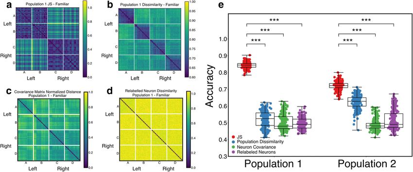
76 • J. Neurosci., January 6, 2021 • 41(1):73–88                                                                                                  Theilman et al. · Topology of Auditory Representation

Figure 1. NCM population activity produces nontrivial topological features. a, Spectrogram from a typical 6 s stimulus with motif boundaries marked with black dotted lines. b, Spike raster
from 100 units from region NCM during one trial of the presentation of the stimulus in a. c, Normalized average Betti curves from the population in b for the stimulus in a. The values of the
Betti numbers are normalized to their maximum during the stimulus presentation, to facilitate visualization of all dimensions on the same plot. The Betti curves are averaged over 20 presenta-
tions of the same stimulus. d, Schematic of the temporal filtration. Beginning with the start of the stimulus, the elementary simplex from each time bin is added to the growing simplicial com-
plex. At each time bin, the Betti numbers for the entire complex up to that point in time are computed. Then, the next bin is added, and the values of the Bettis are recomputed. e, Betti
curves for Betti numbers 0-3 for all stimuli for all populations. Each color represents a different stimulus, and identical colors across panels represent the same stimulus. Shaded regions repre-
sent SEM. Individual stimuli produce unique Betti curves. Betti curves for different stimuli overlap during the first 1 s of the stimulus, consistent with the first 1 s of all stimuli being identical.

    Spatiotemporal structure in population responses to stimuli reflects                              individually and independently within a single trial for each stimulus,
two kinds of correlation. The first is correlation between individual cell                            applying the same bin-to-bin permutation to all trials of that same stim-
spike trains and individual stimuli. We call this the stimulus specificity                            ulus. This creates a new, independent, stimulus-specific response for
of single-unit responses. The other kind of correlation is the set of n-                              each neuron, and replaces the empirical n-wise population correlations
wise correlations between neurons on a single trial across time (some-                                with a random pattern of coactivity that repeats across repetitions of
times referred to as the noise correlation). The fully shuffled condition                             each stimulus.
destroys both these forms of correlation, by assigning different single-                                  Stimulus specificity. We analyzed the stimulus specificity of the em-
unit spike trains, and therefore a random n-wise correlation structure, to                            pirical and shuffled Betti curves by first computing the distribution of
each neuron on each presentation of each stimulus. To dissociate these                                the correlations between the Betti curves of pairs of trials. Then we com-
two correlation sources, we created an additional shuffle of the popula-                              pared the distributions of correlations from a pair of trials within a single
tion data, termed the “within-stimulus mask shuffle,” in which each                                   stimulus to correlations from pairs of trials between different stimuli.
stimulus is associated with a unique time bin-to-time bin permutation                                 The significance of these differences was computed using a linear mixed-
mask. We then shuffle the spiking response of each neuron in time                                     effects model (Lindstrom and Bates, 1988). The model predicted the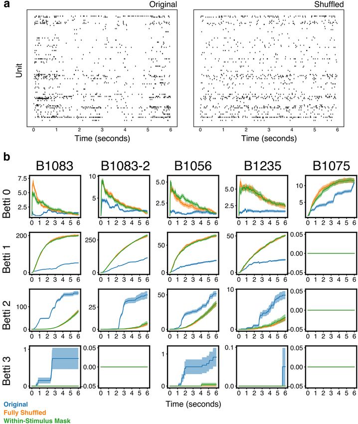
Theilman et al. · Topology of Auditory Representation                                                                       J. Neurosci., January 6, 2021 • 41(1):73–88 • 77

correlation between Betti curves on pairs of trials treating the within-            desirable because these measures should depend only the neural activity
stimulus versus between-stimulus distinction as a random effect and                 and not the specific labels assigned to neurons, analogous to how differ-
treating the average firing rate and an interaction of firing rate and pair         ent maps of the world describe the same geography with different coor-
type as fixed effects. We included firing rate effects since the shuffles pre-      dinates. This definition of JS and KL divergence ignores the eigenvectors
serve average firing rate but destroy precise temporal correlations.                of r and s . Indeed, r and s may not be simultaneously diagonalizable
    Simplicial configuration model. To test whether the topology of the             (or even of the same dimension). Rectifying these issues requires a
neurally derived simplicial complexes is likely to be seen in a random              choice in the definition of the metrics, which like any other metric is
simplicial complex, we used the simplicial configuration model (Young               justified by its ultimate use. We explain our choices in the following
et al., 2017). Because of the computational constraints of the configura-           paragraph. Regardless, the eigenspectra of r and s do form discrete
tion model, for each stimulus, we averaged the neural activity over trials          probability distributions, and the definitions of KL and JS divergence
to yield an average population spike train. The simplicial complex for              here agree with the usual definitions of these divergences on discrete
this spike train was computed and seeded the simplicial configuration               probability distributions.
model software (Young et al., 2017). This algorithm produces a Markov                   One limitation in the naive generalization of the foregoing metrics to
chain that yields samples from the uniform distribution over all simpli-            neural data are that they rely on the density matrices being square and of
cial complexes with local connectivity structure identical to the seed              the same dimension. For real data, however, different stimuli or repeti-
complex derived from neural activity. For each sample, the Betti num-               tions of the same stimulus often evoke different numbers of active neu-
bers were computed using Perseus. The distribution of these Betti num-              rons, giving rise to chain groups, boundary operators, and density
bers serves as a null distribution against which Betti numbers derived              matrices of different dimension. To address this, given two Laplacians
from the empirical data can be compared. We interpret data having Betti             of different dimensions, we expanded the dimension of the smaller
numbers that fall well outside the null distribution as containing nonran-          Laplacian by padding with zeros. An alternative approach is to collapse
dom topological structure. To quantify how far outside the null distribu-           the two simplicial complexes together along their common simplexes
tion an observed Betti number falls, we calculated empirical p values               and derive “masked” boundary operators that only operate on the sim-
using the formula as follows (Davison and Hinkley, 1997):                           plexes within the original, individual complexes, and then define the
                                                                                    Laplacians using these masked boundary operators. Both the “zero-pad-
                                              P                                     ding” and the “masking” approaches yielded similar results for our data-
                                        11      ðbi . be Þ
                                 p ¼                                          (1)   sets. We report results from the computationally simpler method of
                                               N11
                                                                                    zero-padding. In all analyses, the simplicial Laplacian was computed
                                                                                    from the final simplicial complex constructed from the population
     Where bi represents the Betti number for the i-th sample from the sim-
                                                                                    response to an entire trial.
plicial configuration model, N is the number of samples from the simplicial
                                                                                        Beta parameter. The free parameter, b , that appears in the expres-
configuration model, and be is the empirically observed Betti number.
                                                                                    sion for the density matrix originates in statistical physics, where it is
     Simplicial Laplacian. We generalized the methods of De Domenico
                                                                                    interpreted as “inverse temperature,” i.e., b is proportional to 1/temper-
and Biamonte (2016) to define information-theoretic quantities related
                                                                                    ature. The significance of b in the context of network theory is actively
to simplicial complexes. Equipped with the boundary operator matrices
                                                                                    under study (Nicolini et al., 2018). Here we interpret b by noting that it
@i , the simplicial Laplacians (Horak and Jost, 2013) were computed as
                                                                                    acts to normalize the Laplacian matrix, and by extension, the eigenvalues
follows:
                                                                                    of the Laplacian. In this sense, b acts as a “scale parameter” that sets the
                                                                                    scale of the spectral features of interest. The eigenvalues of the Laplacian
                                 Li ¼ @ip @i 1 @i 1 1 @ip1 1                  (2)   are always non-negative; and if b is large, then large eigenvalues are sig-
                                                                                    nificantly damped by the negative exponential. Heuristically, increasing
    where p indicates the adjoint, which in these analyses means the ma-            b decreases the proportion of larger eigenvalues that contribute to the
trix transpose. Given a simplicial Laplacian Ln , the related density matrix        quantities of interest. In our case, if b is too large, too little of the spec-
was computed as follows :                                                           trum will be relevant for the JS or KL divergences, and we reasoned the
                                                                                    results would be less interpretable. To confirm this exponential damping,
                                               eb Ln                               we computed the proportion of eigenvalues above a threshold of 1e-14
                                      rn ¼                                    (3)
                                                                                    as b varied from 0.1-100. Generally, this proportion started decreasing
                                              Tr eb Ln
                                                                                    from 100% with b ffi 1, to below 20% when b . 10. We set b = 1 in all
where b is a free parameter. Given a density matrix expressed in its ei-            of our analyses, but the main conclusions do not change as along as b
gen-basis, the eigenvalues represent the probability distribution over              was below the upper bound of 10.
eigenstates with maximum entropy under the Hamiltonian given by the                     Simulated spiking populations. We used synthetic spike trains to
Laplacian. We can define the Kullback-Leibler (KL) divergence between               examine how well the proposed metrics reveal invariant properties
any two such density matrices, r and s ; by first diagonalizing both r and          between neural populations. For “target” spike trains, we simulated a
s and then sorting each vector of eigenvalues by magnitude. The KL                  population of 20 Poisson spiking neurons for 1000 time-steps with a rate
divergence is then defined by the following:                                        parameter selected from the set (0.01, 0.02, 0.03, 0.04). We generated
                                                                                    “test” spike trains by choosing 50 rate parameters evenly in the range of
                                        X                                           [0.001, 0.1] and simulating 25 population spike trains for each rate. We
                     DKL ð r ; s Þ ¼               r i ðlog r i  log s i Þ   (4)   computed the simplicial KL divergence between each test spike train and
                                               i
                                                                                    the target spike train, then computed the average divergence between
   Where r i is the i-th eigenvalue. The Jensen-Shannon (JS) divergence             the target and the model at the given rate parameter.
was defined using the following:                                                        We applied the same procedure to simulate heterogeneous Poisson
                                                                                    populations, except that half of the neurons were simulated with rate pa-
                                                                                    rameter 0.02 and the other with 0.05. The assignment of neurons to rate-
                                                r 1s
                                       M ¼                                    (5)   parameter subgroups was random. The above-described parameter
                                                  2                                 sweep procedure was repeated over the two population rate parameters.
                                                                                        Simulated environments. We simulated physical environments simi-
                                      1                                           larly to the environments used in Curto and Itskov’s original work
                   DJS ð r ; s Þ ¼       DKL ð r ; MÞ 1 DKL ðs ; MÞ           (6)
                                      2                                             (Curto and Itskov, 2008). We randomly placed 0-4 holes of radius 0.3 m
                                                                                    inside a 2  2 m arena, ensuring hole centers did not overlap. We then
   The advantage of sorting the eigenvalues is that the divergence                  randomly distributed 100 place fields of radius 0.2 m in the environment
becomes invariant to the labels assigned to individual neurons. This is             using an algorithm that ensured that the environment was fully tiled. To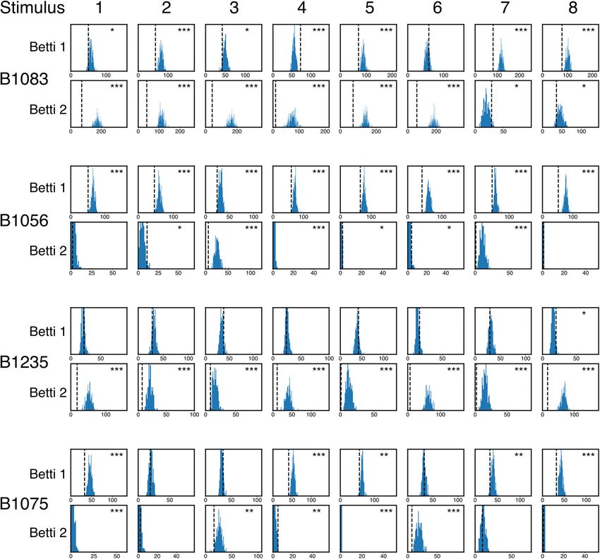
78 • J. Neurosci., January 6, 2021 • 41(1):73–88 Theilman et al. · Topology of Auditory Representation
model movement, we constructed a random walk trajectory simulating a whether a pair of responses to different stimuli came from stimuli that
10 min traverse of the environment sampled at 10 samples per second to belonged to either the same or different behaviorally trained class based
ensure the whole arena was explored. We constructed spike trains by on the value of either the JS divergence or the specific correlation mea-
simulating Poisson spike trains at a constant rate for each neuron while sure of interest between the responses. Regressions were fit to a random
the random walk trajectory was within the cell’s place field, and silent subset of 80% of the data and tested on the remaining 20%. A total of
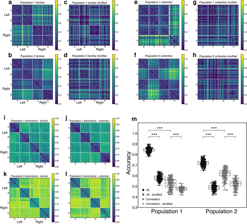
outside of it. 240 separate regressions were performed for each condition.
We constructed five different environments with each specified We measured the similarity of topological structure across disjoint
number of holes. For each environment, 10 random walks were simu- subpopulations by randomly splitting the full dataset from B1083
lated. The pairwise 1-JS divergence between pairs of individual trials was Population 1 into two disjoint subgroups each with 50 neurons. Then we
computed by taking the simulated spike trains’ 1-Laplacians and com- conducted an identical analysis to the logistic regression described in the
puting the spectral JS divergence as defined above. We averaged the 1-JS preceding paragraph but using the JS divergence between responses
divergences over all walks for each environment to yield the plot in from the two disjoint populations. We repeated this 40 times with a dif-
Figure 5a. Then, the JS divergences for each of the 25 environment pairs ferent (randomly chosen) split of the original population. We assessed
with given numbers of holes were averaged to yield the plot in Figure 5b. the difference between the means of the accuracies of the regressions fit
In vivo JS divergences. Data from trained, anesthetized birds was to the JS divergence or correlations with a Gaussian GLM from the stats-
recorded and preprocessed to yield population spike trains as described models python library with the type of measure (JS divergence/correla-
earlier. The JS divergence analyses were restricted to the four learned tion) and the type of shuffle (shuffle/no shuffle) as regressors, and
stimuli and four other unfamiliar stimuli. For an arbitrary pair of included an interaction term between the shuffle and measure.
responses from two separate stimulus presentations, the 1-Laplacian of Linear mixed-effects model. We used a linear mixed-effects model to
each response was computed by first converting the neural data into a examine the stimulus specificity of the empirically derived Betti curves
simplicial complex as described above, using a bin size of 10 ms with associated with each stimulus, and those derived from the various shuf-
5 ms overlaps. Then, the JS divergences between the 1-Laplacians were fled versions of the spiking responses. The regression models predicted
computed as described above. It is important to note that the JS diver- the correlation between Betti curves in a given dimension between pairs
gences were computed using the final simplicial complex from each trial. of trials, as a function of whether the pair came from two trials of a single
As a result, it may “miss” homological features that do not persist stimulus or two trials of different stimuli. The model included popula-
through the whole trial. We do not consider this a limitation in the pres- tion identity as a random effect. The model was implemented using
ent study, since the final simplicial complex reflects the aggregate effects MixedLM from the statsmodels python library. We included firing rate
of temporal coactivations through the entire trial, and thus tells us some- (and its interaction with stimuli) as a separate fixed effect in the model
thing about the population response to the entire stimulus considered as and exclude this from all reported effects on Betti curve correlations tied
a unit. Nevertheless, it will be valuable for future work to explore the to stimulus specificity. Overall, the mean firing rate on a pair of trials
properties of these features that may be missed by the current analysis. tends to increase the strength of the correlation between Betti curves on
Correlation-based population response similarity. As an alternative those trials, in part because it tends to smooth over small moment-to-
to the simplicial Laplacian spectral entropy (SLSE) measure of popula- moment variations in a manner equivalent to computing simplicial com-
tion similarity, we also compute a correlation-based measure to quantify plexes from spike trains quantized into larger time bins.
the trial-to-trial similarity in the response of a population, C(A,B), where
A and B are the responses of the same population on different trials
responding to either the same stimulus or to different stimuli. We first Results
smooth the population spike trains with a Gaussian kernel with a width Stimulus-specific topological structure in auditory neural
of 10 ms, then compute the correlation coefficients between the spike populations
train of a neuron in response A and the spike train from the same neu- We first asked whether auditory stimulus-driven NCM popula-
ron in response B, then average across all the correlation coefficients to a tion activity can be well described by its spike-based topological
yield a raw scalar estimate of similarity, C, between the two populations. structure. We recorded song-evoked responses from five, dis-
We use 1 – C in place of the raw correlation measure so that smaller val-
tinct, large populations of neurons in the NCM of adult starlings
ues of both correlation and JS divergence indicated more similar spike
trains, such that 1 – C = 0 when the response of every single neuron in (323 neurons total, distributed across 4 birds; B1083: 101, 95
the population for population response A is perfectly correlated with its neurons in two separate populations; B1056: 54; B1235: 40;
corresponding response for population response B. Comparing this sim- B1075: 33). For each presentation of each song stimulus within
ilarity measure with the SLSE measures allows us to test whether physi- each population, we rerepresented the full population spike train
cally dissimilar responses (in terms of the actual spike trains) may evince as a simplicial complex, then computed the Betti curves (see
similar topologies. Materials and Methods) associated with each song stimulus.
We also compute the distance between pairs of population responses Each Betti curve describes structure in the population coactivity
using covariance matrices. For each trial, we calculated the pairwise co- pattern across time. More specifically, each curve captures the
variance matrix between Gaussian-smoothed spike trains, again with a
evolution of the homology of the simplicial complex in a single
10 ms window. This yields an N_cell N_cell matrix for each trial in
which each i,j entry is the temporal covariance between the smoothed dimension, as defined by the time-resolved spiking pattern
spike trains from neurons i and j on that trial. We obtained a distance across each neural population for a given stimulus (Fig. 1).
between pairs of trials by computing the Frobenius norm of the differ- Visual inspection of the trial-averaged Betti curves (Fig. 1e) sug-
ence between each trial’s covariance matrix. The distance matrix was gests consistent stimulus-specific temporal dynamics in the
normalized by its maximum value over all pairs of trials to yield a nor- homology of Dimensions 0, 1, and 2. Although the simplicial
malized distance measure. This measure places two trials close to each complexes sometimes display 3-dimensional homology (Fig. 1e,
other if the second-order (pairwise) correlation structure in the popula- bottom row), these are not consistent across birds or stimuli. We
tion for response A is similar to the second-order correlation structure note that the trajectories of the Betti curves in Dimensions 0-2
for response B.
tended to overlap during the first motif for each stimulus, con-
The correlation between population responses with relabeled neu-
rons was obtained by shuffling the rows of the Gaussian smoothed popu- sistent with their stimulus specificity, as the first motif was the
lation response matrix and repeating the population correlation same for all songs.
computation described above on the shuffled matrices. Betti numbers provide one measure of topological properties
JS divergence and correlation measures were compared using the rel- present in the underlying neural population coactivity, and so
ative accuracy of logistic regressions. We fit logistic regressions to predict can be interpreted as abstract proxies for structure. They also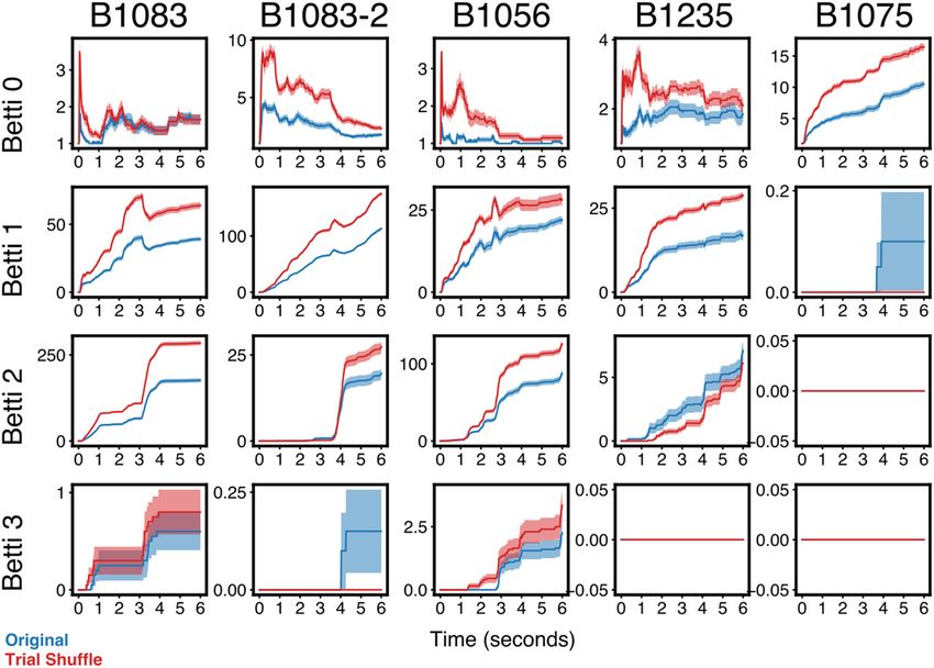
Theilman et al. · Topology of Auditory Representation                                                                             J. Neurosci., January 6, 2021 • 41(1):73–88 • 79

provide insight into more concrete aspects of the underlying            Table 1. Stimulus specificity of empirical and shuffled Betti curvesa
population activity. Betti 0 counts the number of connected com-        Dataset             Betti number         Coefficient      z               p               97.5% CI
ponents in the simplicial complex. Thus, for neural data, increas-
                                                                        Empirical           0                    0.031            4.083         4.45e-05        [0.046, 0.016]
ing Betti 0 suggests multiple independent subsets of neurons
                                                                        Shuffled            0                    0.010            1.275         0.202           [0.024, 0.005]
firing coincidently within a group but not across groups. Higher        Within-mask         0                    0.003            0.33          0.741           [0.017, 0.012]
dimensional Betti numbers, 1 to N, count the number of n-               Empirical           1                    0.032            5.571         2.53e-08        [0.043, 0.021]
dimensional “holes” in the simplicial complex. For neural popu-         Shuffled            1                     0.000             0.303         0.762           [0.003, 0.004]
lation coactivity patterns, the Betti n count corresponds loosely       Within-mask         1                     0.002             1.432         0.152           [0.001, 0.005]
to the number of gaps (i.e., periods of simultaneous inactivity         Empirical           2                    0.149           15.603         6.96e-55        [0.167, 0.130]
among neurons, or “missing” patterns of coactivity). As these           Shuffled            2                    0.030           2.993          0.003           [0.050, 0.010]
gaps fill in, because of coincident activity, the corresponding         Within-mask         2                    0.008           0.857          0.391           [0.027, 0.011]
                                                                        a
Betti numbers may decrease.                                              A linear mixed-effects model was used to compute the dependence of the Betti curve correlation on the
                                                                        type of trial pair (within stimulus or between stimuli). For all Betti numbers, the empirical curves show sig-
    To quantify stimulus specificity, we computed all the correla-      nificant stimulus specificity, and this specificity is abolished by both fully shuffling the spikes and performing
tions between Betti curves from pairs of trials with the same           the within-stimulus mask shuffle (see Materials and Methods).
stimulus and pairs of trials from different stimuli. We defined
the population as being stimulus-specific if the distribution of        many such neurons are therefore also likely to be stimulus-spe-
within-stimulus correlations is significantly larger (i.e., closer to   cific, but the specific pattern of coactivations among individual
1, more similar) than the distribution of between-stimulus corre-       neurons that defines the topology may or may not be determined
lations. By this measure, all Betti curves show significant stimu-      by chance. That is, the topology may reflect random coactivity
lus specificity (linear mixed-effects model, Z  4.083 p              between independent spike trains driven by individual stimuli
4.45e-5 for all dimensions), with the coefficient significantly less    (i.e., the stimulus specificity of single-unit responses), and/or a
than zero (Table 1), indicating that between-stimulus correla-          unique nonrandom n-wise pattern of coactivity between neurons
tions are significantly lower than within-stimulus correlations.        that is associated with a given stimulus, where n ranges from 2 to
That is, the topology of auditory stimulus-driven population ac-        the number of recorded neurons. The full-shuffle destroys both
tivity in NCM is stimulus-specific.                                     these forms of coactivity by permuting single unit spike trains on
    To further characterize the stimulus-specific dynamics of the       each presentation of each stimulus, which in turn yields a unique
Betti curves and examine the source of the stimulus specificity in      n-wise coactivity structure on each trial. To further investigate
the empirical population response, we compared the original             these two possible sources of population coactivity structure, we
Betti curves with those obtained after shuffling the spiking            created an additional shuffle of the original population data
                                                                        using a “shuffle mask” that describes how to permute the time
response of each neuron in time individually and independently,
                                                                        bins for a given neuron on a single trial. We randomly generated
within each trial (see Materials and Methods). This shuffle,
                                                                        a shuffle mask independently for each stimulus, and then applied
which we call the full-shuffle, preserves the total number of
                                                                        the same mask to all trials from a single stimulus. This creates a
spikes and spike rate per trial, but destroys all the original spike-
                                                                        new random correlation pattern between the spike trains of indi-
time coincidences between neurons in the population. Because            vidual neurons and individual stimuli, and a random n-wise
the topological structure of the population depends on the spike-       coactivity pattern between individual neurons, that are both pre-
time coincidences, any stimulus specificity tied explicitly to the      served across separate trials from the same stimulus. If the
spike-time based topology (rather than the overall spike rate)          observed stimulus-specific topologies emerge from a random
should be abolished in the full-shuffled data. This in turn should      alignment of spiking responses repeated across trials of the same
yield Betti curves that are more similar across different stimuli       stimulus, the mask-shuffled data should resemble an empirical
and birds compared with the original Betti curves. Figure 2             response to a novel stimulus. If, however, the empirical n-wise
shows the Betti curves that result from the full-shuffle (in orange)    correlation structure is privileged in some way, then the mask-
for a single stimulus from each of the populations. In each             shuffled data should resemble the full-shuffle responses.
dimension, the fully shuffled curves show a degeneration to a               We recomputed the Betti curves for the within-stimulus
stereotypical trajectory across populations. The same pattern is        mask-shuffled data. Figure 2 shows the various shuffled Betti
observed for all other stimuli. We quantified this explicitly by        curves from an arbitrarily chosen stimulus for each population.
again comparing correlations between Betti curves from pairs of         Like the full-shuffle, the Betti curves for the mask-shuffled data
trials within and between stimuli. For Betti 0 and 1, the shuffled      do not appear to be stimulus-specific. To test this, we again
curves were not stimulus-specific (linear mixed-effects model,          measured stimulus specificity by computing the distributions of
p . 0.202). For Betti 2, some marginal stimulus specificity             correlations between pairs of Betti curves from trials with either
remained (linear mixed-effects model, Z = 2.993, p = 0.003),           the same or different stimuli. The mask-shuffled Betti curves did
but the magnitude of the specificity was significantly smaller          not show significant stimulus specificity (linear mixed-effects
than that for the empirical data (linear mixed-effects model, Z =       model, p . 0.152 for all Betti numbers). Table 1 gives the results
21.24, p , 1e-13). Based on these results, we conclude that the        of the linear mixed-effects model (see Materials and Methods)
topological structure of NCM population activity reveals stimu-         that assesses the significance of stimulus specificity in the Betti
lus-specific coincident patterns of neuronal firing.                    curves from the within-stimulus mask shuffle. Figure 3 presents
    How is it that the temporal coactivity pattern of the popula-       histograms of the Betti curve correlations for within-stimulus
tion response, as measured by the topology, carries stimulus-spe-       and between-stimulus pairs of trials, for both the empirical and
cific information? One possibility is that the population simply        shuffled data, for population B1083. The lack of stimulus speci-
inherits specificity from single-unit responses. Individual NCM         ficity in both the full- and mask-shuffled data supports the
neurons have complex receptive fields (Kozlov and Gentner,              conclusion that stimulus-evoked coactivity in NCM carries stim-
2016), and their responses are likely to be stimulus-specific           ulus-specific information that is not a trivial product of ran-
(Thompson and Gentner, 2010). The collective responses of               domly aligned stimulus-specific single-neuron responses.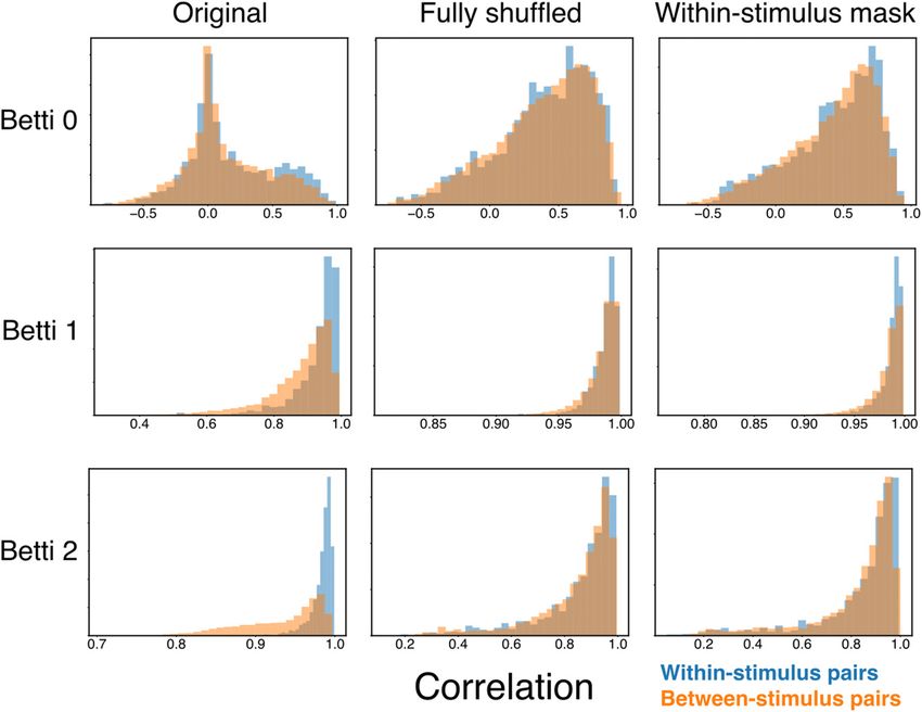
80 • J. Neurosci., January 6, 2021 • 41(1):73–88                                                                                            Theilman et al. · Topology of Auditory Representation

Figure 2. Shuffled Betti curves. a, Example empirical and shuffled population responses from an example trial. b, The average Betti curve for Dimensions 0-3 from an example stimulus is
plotted for all populations. The empirically observed Betti curves (blue) are obtained from the raw neural data. Control Betti curves are computed from “fully shuffled” (orange) neural data in
which the responses of individual cells are independently shuffled in time (see Materials and Methods), or the same neural data with the single-trial spike responses permuted by either a
within-stimulus mask (green) or across trials (red). A different within-stimulus mask was generated for each stimulus, and the same mask was used for all trials of a given stimulus. The shuf-
fled curves strongly overlap and are significantly different in shape and magnitude from the empirical Betti curves. Shaded regions represent SEM.

    The differing shapes of the Betti curves for the empirical and                                    As noted, the topological analyses we detail differ in funda-
both the full- and mask-shuffled spike trains suggest that the                                    mental ways from traditional correlation-based measures of pop-
NCM population activity is structured nonrandomly at scales                                       ulation coactivity. Nonetheless, it is helpful to understand our
above the single neuron. To test this idea directly, we asked how                                 results within the context of classically defined noise correlations
likely it is that the observed topological structure in a given pop-                              (i.e., the stimulus-independent covariance in simultaneous firing
ulation might occur by chance. We constructed a null model for                                    rates between neurons). To do this, we again shuffled the empiri-
simplicial complexes that produces samples from the uniform                                       cal data, this time by permuting spikes across trials rather than
distribution over all simplicial complexes that match the “local                                  time. The Betti curves for these trial-shuffled data show similar
structure” of a given “seed” complex (Young et al., 2017), and                                    trajectories compared with those for the empirical data (Fig. 5),
used this model as the basis to compare the final Betti numbers                                   but with larger magnitudes. This suggests that the relative tem-
for each stimulus (Fig. 4). For each bird, the majority of the stim-                              poral dynamics of the coactivity pattern are governed largely by
uli showed responses with at least one Betti number significantly                                 what would be referred to, classically, as the “signal correlation,”
outside the null distribution (B1083: 8 of 8 stimuli; B1056: 8 of 8                               whereas the absolute number of “holes” in a given topological
stimuli; B1235: 8 of 8 stimuli; B1075: 7 of 8 stimuli). Thus, the                                 dimension is constrained by the “noise correlation.” The magni-
stimulus-specific topology in NCM population spiking is not                                       tude of Betti n corresponds roughly to the number gaps in the
produced by chance spike coincidences between neurons.                                            population responses that are bounded by coactive cell groups of
Theilman et al. · Topology of Auditory Representation J. Neurosci., January 6, 2021 • 41(1):73–88 • 81
the reasoning that it could be used simi-
larly to fit the parameters of spiking
neural network models. To test this rea-
soning, we began with a proof of con-
cept: fitting the rate parameter of a
simulated population of Poisson-spiking
neurons. The population consisted of 20
neurons each firing independently and
with a rate parameter that was constant
across the population. We simulated a
single trial of 1000 time samples to serve
as the “target” population spike train.
We then performed a parameter sweep
by simulating the population with a rate
parameter that varied in some range.
For each choice of rate parameter, 25
“test” trials from the model were simu-
lated and the 1-KL divergence between
the “target” population spike train and
each “test” trial population spike train
was computed. The 1-KL divergences
from each of the 25 trials of the chosen
parameter were averaged together.
Figure 6a displays the 1-KL divergence
Figure 3. Example Betti curve correlation distributions. Stimulus selectivity of the Betti curves is assessed by computing the as a function of the test rate parameter
distributions of the pairwise correlations between Betti curves on pairs of trials. Shown are distributions from bird B1083. Blue for four different models with different
distributions come from trial pairs that belonged to the same stimulus. Orange distributions come from pairs that belong to dif- “target” rate parameters. The dotted
ferent stimuli. The original, empirical distributions show significant differences, indicating stimulus selectivity of the Betti
lines indicate the true value of the rate
curves. The distributions computed from shuffled data show little difference among within or between stimulus pairs. The sig-
nificance of the differences in these distributions was assessed using a linear mixed-effects model. Table 1 lists the significance parameter used to generate the target
for the empirical, fully shuffled, and within-stimulus mask shuffled conditions. population spike train for each model,
separated by color. For each model, the
minimum of the KL divergence closely
approximates the true value of the rate
order n; and as these gaps fill in, Betti n decreases. In other parameter.
words, noise correlations increase the numbers of coactive cell We next tested a slightly more complicated model that had
groups. Overall, both the signal and noise correlation contribute two distinct populations of neurons. Each population was again
to the topological structure of coactivity on each trial. This is Poisson, but the two populations had differing rate parameters.
consistent with previous studies (Jeanne et al., 2013) that show Figure 6b shows a heat map plotting the 1-KL divergence as a
NCM signal and noise correlations are not independent. function of the two rate parameters. The white dots indicate the
true parameters. There is a degeneracy in this model in that it
Topological tools for comparing population spiking activity does not matter which subpopulation is labeled A and which is
Representing population spiking activity with a simplicial com- labeled B. Again, the minima of the 1-KL divergence closely ap-
plex has the advantage of providing a single mathematical object proximate the true values of the parameters for the heterogene-
that encodes the entirety of the spatiotemporal structure of the ous population.
population response on a single trial. This entity is non-numeri- Importantly, for all of the Poisson spike train simulations, the
cal, however; and so to facilitate numerical comparisons, we “test” and “target” spike trains never coincided. Instead, similar-
sought to define a numerical measure of similarity between sim- ities quantified by the simplicial KL divergence rely on the global
plicial complexes. To do this, we generalized recent advances in topological structure of the population spike trains, not on the
network theory to define information-theoretic measures of sim- match between specific spike trains of single neurons. The SLSE
plicial complex structure and similarity. A detailed description of is sensitive to how the activity of an individual neuron relates to
these measures is provided in Materials and Methods; Table 2 the simultaneous activity of all the other neurons in the popula-
gives the principle formulas in this analysis. We refer to this gen- tion in which it is embedded.
eral approach of computing information theoretic quantities
from simplicial complexes as SLSE. Reconstructing latent stimulus relationships using SLSEs
Our observation that NCM populations produce nonrandom,
Fitting spiking models using SLSE stimulus-specific, topologies implies that Poisson spike trains are
The KL divergence is often used as a cost function for statistical not a good source of biologically relevant topologies, and so the
model fitting, in which one attempts to choose the parameters of above evaluation of these metrics is limited. As a more biologi-
a statistical model such that the model distribution is as close to cally relevant validation of the SLSE measures, we turned to the
the data distribution as possible. The KL divergence can be place cell system used in the original Curto and Itskov (2008)
defined to allow for this same sort of model fitting, but for graphs study of neural population-derived simplicial complexes and
(De Domenico and Biamonte, 2016). We extended the KL diver- began by replicating these earlier results. We simulated the activ-
gence to simplicial complexes (see Materials and Methods) with ity of hippocampal place cells during free exploration of aYou can also read