Stable Fast Rewiring Depends on the Activation of Skeleton Voxels
←
→
Page content transcription
If your browser does not render page correctly, please read the page content below
Stable Fast Rewiring Depends on the Activation
              of Skeleton Voxels

                          Sanming Song and Hongxun Yao∗

     School of Computer Science and Technology, Harbin Institute of Technology,
                              150001, Harbin, China
                           {ssoong,h.yao}@hit.edu.cn

        Abstract. Compared with the relatively stable structural networks, the
        functional networks, defined by the temporal correlation between remote
        neurophysiological events, are highly complex and variable. However, the
        transitions should never be random. So it was proposed that some stable
        fast rewiring mechanisms probably exist in the brain. In order to probe
        the underlying mechanisms, we analyze the fMRI signal in temporal di-
        mension and obtain several heuristic conclusions. 1) There is a stable
        time delay, 7∼14 seconds, between the stimulus onset and the activation
        of corresponding functional regions. 2) In analyzing the biophysical fac-
        tors that support stable fast rewiring, it is, to our best knowledge, the
        first to observe that skeleton voxels may be essential for the fast rewiring
        process. 3) Our analysis on the structure of functional network supports
        the scale-free hypothesis.

        Keywords: fMRI, rewiring, functional network.

1     Introduction
Though ∼3×10⁷ synapses are lost in our brain each year, it can be neglected
when taking the total number of synapses, ∼1014 , into consideration. So the
structural network is relatively stable. But the functional networks, which relates
to the cognitive information processing, are highly variable. So a problem aris-
ing: how does a relatively stable network generate so many complex functional
networks? It has puzzled intellects for years [1]. We don’t want to linger on this
enduring pitfall, but only emphasize the functional network, especially the tran-
sition between functional networks. For, though incredible advances have been
obtained in disclosing the structural network with the help of neuroanatomy, we
know little about the functional networks [2].
   Gomez Portillo et al. [3-4] recently proposed that there may be a fast rewiring
process in the brain, and they speculated that the scale-free characteristics might
be determined by a local-and-global rewiring mechanism by modeling the brain
as an adaptive oscillation network using Kuramoto oscillator. But their assump-
tions are problematic. Since human cognitions are continuous process, the ran-
dom assumption about the initial states is infeasible. What’s worse, the rewiring
∗
    This work is supported by National Natural Science Foundation of China (61071180).

B.-L. Lu, L. Zhang, and J. Kwok (Eds.): ICONIP 2011, Part I, LNCS 7062, pp. 1–8, 2011.

c Springer-Verlag Berlin Heidelberg 2011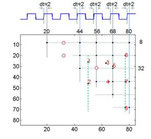
2       S. Song and H. Yao

          (a)                       (b)                           (c)

Fig. 1. Morphological dilation to ROI: (a) the activated region given by SPM; (b) the
extracted ROI; (c) the mask obtained by ROI dilation

is too slow to satisfy the swift and precise information process requirements
of the brain. (Also, in personal communication, Gomez Portillo explained that
the underlying biophysical basis is not clear at present.) Obviously, our brain
has been experiencing ”oriented” rewiring instead of “random” rewiring, so the
rewiring is stable, and which should be oriented to response precisely to the
stimulus.
   To disclose the biophysical mechanisms underlying fast rewiring, we conduct
explorative analysis to the fMRI signal in temporal dimension and many impor-
tant and heuristic conclusions are drawn. The experiment material is introduced
in Section 2. In Section 3 and 4, we analyze the temporal stability and skeleton
voxels. Finally, we conclude this paper in Section 5.

2   Material
Analysis were conducted based on an auditory dataset available at the SPM site
[5], which comprises whole brain BOLD/EPI images and is acquired by a mod-
ified 2 Tesla Siemens MAGNETOM Vision system. Each acquisition consisted
of 64 contiguous slices (64×64×64 3mm×3mm×3mm voxels). Data acquisition
took 6.05s per volume, with the scan to scan repeat time set to 7s. 96 acqui-
sitions were made (TR=7s) from a single subject, in blocks of 6, giving 16 42s
blocks. The condition for successive blocks alternated between rest and auditory
stimulation, starting with rest. Auditory stimulation was with bi-syllabic words
presented binaurally at a rate of 60 per minute [6]. The first 12 scans were dis-
carded for T1 effects, leaving with 84 scans for analysis. SPM8 was the main tool
for image pre-processing. All volumes were realigned to the first volume and a
mean image was created using the realigned volumes. A structural image, ac-
quired using a standard three-dimensional weighted sequence (1×1×3mm3 voxel
size) was co-registered to this mean (T2) image. Finally all the images were spa-
tially normalized [7] to a standard Tailarach template [8] and smoothed using a
6mm full width at half maximum (FWHM) isotropic Gaussian kernel. And we
use the default (FWE) to detect the activated voxels.

3   Temporal Stability
Though SPM can be used to detect the activated regions, as shown in Fig.1
(a), we know little on the temporal relationship between the stimulus and the
Stable Fast Rewiring Depends on the Activation of Skeleton Voxels 3
(a) (b)
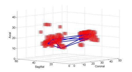
Fig. 2. The temporal stability of fast rewiring. For convience, only the upper triangle
part of the binary similarity matrix is show, and the threshod coefficients are (a)η =
0.4,(b)η = 0.5. The rectangle wave above each matrix denotes the stimulus onset in
the block design. The local maximum (denoted by black dots) show that there is a
huge jump between the first and the second scan after each stimulus onset. And the
periodicality of local maximums, which is consistent with the periodicality of stimulus
onset, shows that the delay between the stimulus onset and the corresponding cortical
activation is very stable. And the delay is about 7 14 seconds (dt=2 scans, TR=7
seconds). Not that there are some “noise”, like the missing of local maximums (red
circles) or priming phenonmenon (red numbers), please see the text for explainations.
response. So, in order to facilitate the analysis, we need to extract those activated
voxels for post-processing. And the extracted activated regions, also known as
region of interest (ROI), is shown in Fig.1 (b).
The ROI provided by SPM are the most activated voxels responding to the
stimulus. In order to reduce the noise and also facilitate the latter analysis, we
expand the ROI at firstly, because the essential voxels that play an important
role in rewiring may be not included in the ROI, as it shown in latter sections.
We adopt the morphological dilation [9]and the 3×3×3 cubic structural element
is used. The dilated ROI, denoted as M , is shown in Fig.1 (c).
Due to the adaptation effects or the descending of blood oxygenated level
of the functional regions, the energy intensity of fMRI signal varies with large
amplitude. To facilitate the comparison between scans, we have to normalize the
energy of eachscan. Let fi be the ith scan, and gi be the normalized image, then
the normalization can be depicted as
max {fi }
i
gi = fi (1)
fi
where · stands for the mean energy. Then we can extracted the voxels of
interests using the mask M ,
Gi = [gi ]M (2)
where Gi is the masked image.4 S. Song and H. Yao
Even when the brain is at the resting state, the intensities of voxels are very
large. So the baseline activities of voxels are very high, and the stimulus only
makes the voxels more active or less active. Compared with the mean activities,
the energy changes are very small, so it is better not to use the original voxels
intensities. We differentiate the images as follow,
dGi = Gi − Gi−1 (3)
By the way, the baseline activity of each voxel is described by a constant factor in
the design matrix. Threshold the differential images with some θ and transform
the images into binary vectors, then we can obtain the similarity matrix by
calculating the inner product of any two binary vectors. That is,
dist (Gi , Gj ) = sgn (dGi − θ) , sgn (dGi − θ) (4)
where θ = η · max {dist (Gi , Gj )}ij and ηis a coefficient.
If the onset of stimulus can induce remarkable change in fMRI signal, there
would be a steep peak in the corresponding differential vector. And if the change
is also stable, then there would be periodic local maximums. In Fig.2, we show
the local maximums using different thresholds. For convenience, we only show the
upper triangle part of the binary similarity matrix. See the caption for details.
As it can be seen from Fig.2, there are periodic local maximums in the sim-
ilarity matrix. So the periodic stimulus can induce the periodic enhancement
and recession of fMRI signal. So the dynamic rewiring of functional network is
temporal stable.
What’s more, we found that the local maximums don’t appear immediately
when the stimulus set, and there is always 2-period delay. Because the scanning
period, 7 seconds, is too large when compared with the cognitive processing
speed of the brain, and the volumes were pre-processed by slice-timing, the
time delay is estimated to be about 7∼14s, which coincides with the theoretical
value [6]. The stable time delay phenomenon reminds us that we can study the
mechanisms and rules underlying the fast rewiring by scrutinizing these first
2-scans after each stimulus onset, which would be described in the next section.
It is also interesting to note that there are two kinds of noise in the similarity
matrix. The first one is the pseudo local maximums, like 1-4 and 6-8 in Fig.2
(a) and 1 in Fig.2 (b). The pre-activation behaviors may be relevant to the
priming phenomenon [10]. By the way, in SPM, these activities are captured by
the derivative of HRF function [11].
The second is the absence of some local maximums. It is worth nothing that
the absences can’t be understood as the deactivation of these regions. There
are two ways to look at the issue: the first is that the results largely depend on
the threshold, with lower ones produces more local maximums; and the second is
that the basic assumption, the brain is at resting state when stimulus disappears,
may not hold some time, due to the activity changes induced by the adaptation
or any physiological noise.Stable Fast Rewiring Depends on the Activation of Skeleton Voxels 5
(a) (b)
Fig. 3. The transition matrix(a) and its eign values(b). Only one eigen value is much
large than other eigen values. So approximately, there exists an linear relationships
between the column of the transformation matrix.
4 Skeleton Voxels
Let Gji be the jth scanned fMRI image after the onset of the ith stimulus. All
the first scans are denoted as G1 = [G11 , · · ·, G1S ], the second scans as G2 =
[G21 , · · ·, G2S ], where S is the number of stimulus. The transition matrix is A,
then
G2 = AG1 , (5)
Using the simple pseudo-inverse rule, we have
T
T −1
A = G2 G1 G1 G1 . (6)
The transition matrix is shown in Fig.3(a). To analyze the characteristics of the
transition matrix, we decompose the matrix by SVD (singular matrix decompo-
sition) and the eigen values are plotted in Fig.3(b). The first eigen value is much
larger than any other eigen values. So the matrix nearly has only one princi-
ple direction. It demonstrates that there is an approximately linear relationship
between the columns. It accords with what we see from Fig.3, the rows of the
transition matrix are very similar, but the columns are very different.
Turn formula (8a) to its add-and-sum form,
K
G2in = anm G1im , (7)
m=1
where anm can be seen as the weight of the m th voxel.
As described in Section 2, there is a rest block before each stimulus onset, so
in statistics, we consider the activity of each voxel to be random. Then formula
(8b) can be simply reduced to
K
G2in ≈ G1i· anm , (8)
m=16 S. Song and H. Yao Fig. 4. Skeleton voxels and the connections between them. Note that the connections are obtained by threshod the connection weights anm . Fig. 5. Voxel Degree follows truncated exponential distribution. Thr stands for differ- ent threshold coefficients. where G1i· stands for the mean energy of the first scan after the onset of the ith stimulus. Then anm can also be seen as the contributions of the mth voxel. As discussed above, the columns of the trasition matrix differs much, so it is probably that only a subset of voxels, which have larger contributions, play essential roles. Threshold the transform matrix shows that only several voxels are very important in function network rewiring, as shown in Fig.4. We named them “skeleton voxels”. Similarly, anm can be seen as the connection weight between voxel m and n . If we threshold the weight and only take the presence or absence of these connec- tions into consideration, the degree distribution of voxels can also be obtained. As shown in Fig.5, the degrees follow a truncated exponential distribution, which supports the conclusion of Achard et al. [12]. It says that only a small subset of voxels have large degree, while the others have small degree, and which is the typical characters of scale-free network. We also found that most of the voxels with large degree belong to skeleton voxels, so skeleton voxels might support stable fast rewiring by widespread connections. We also analyzed the neighbor distribution of single voxels. In most cases, their activations are mainly determined by few local neighboring voxels and
Stable Fast Rewiring Depends on the Activation of Skeleton Voxels            7

their counterparts in the opposite hemisphere, which supports the sparse coding
hypothesis and the connection role played by the callose. A sample is shown in
Fig.6. It should be noted that skeleton voxels have more neighbors, and we think
it may have something to do with the stability requirements.
   Of course, the “closest” neighbors correlate with the specific tasks brain un-
dertakes. But our analysis shows that some voxels may be essential for the stable
fast rewiring.

5    Discussions and Conclusions
Our brain experiences complex changes every day. When stimulus set, peripheral
sense organs send information into the central neural system. Then we formu-
late the cognition by functional complex network dynamics [13]. Cognition to
different objects or concepts relies on different functional works. So analyzing the
switching mechanisms between networks is not only essential for disclosing the
formulation of function networks, but also for revealing the relationship between
structural network and function networks. They are all heuristic for artificial
networks.
   The emergence of fMRI technology provides us the opportunity to analyze
the network mechanisms in a micro-macro scale. The paper mainly discusses the
stability of fast rewiring in functional network by analyzing the fMRI signal, and
many interesting and heuristic conclusions are drawn. Firstly, we verified that
there is a 2-scans time delay between the stimulus onset and the activation of
corresponding functional region. The most important is that we found that the
delay is very stable. Secondly, we proposed for the first time that there might be
skeleton voxels that induces the stable fast rewiring. What’s more, our analysis
on the degree distribution of voxels supports the scale-free hypothesis.
   Also recently, we note that Tomasi et al [14][15] proposed that some “hubs”
areas are essential for the brain network architecture by calculating the density of
functional connectivity. Our analysis supports their conclusions. But our method
provides a new way to analyze the activation pattern of each sub-network. Our
future work will focus on the statistical test of skeleton voxels, exploration of
skeleton voxels in other modals and reasoning the origination skeleton voxels.

Acknowledgments. We thank Welcome team for approval use of the MoAE
dataset. Special thanks go to He-Ping Song from Sun Yat-Sen University and
another two annoymous viewers for their helpful comments for the manuscript.

References
 1. Deligianni, F., Robinson, E.C., Beckmann, C.F., Sharp, D., Edwards, A.D., Rueck-
    ert, D.: Inference of functional connectivity from structural brain connectivity. In:
    10th IEEE International Symposium on Biomedical Imaging, pp. 460–463 (2010)
 2. Chai, B., Walther, D.B., Beck, D.M., Li, F.-F.: Exploring Functional Connec-
    tivity of the Human Brain using Multivariate Information Analysis. In: Neural
    Information Processing Systems (2009)
8 S. Song and H. Yao
3. Gomez Portillo, I.J., Gleiser, P.M.: An Adaptive Complex Network Model for Brain
Functional Networks. PLoS ONE 4(9), e6863 (2009),
doi:10.1371/journal.pone.0006863
4. Gleiser, P.M., Spoormaker, V.I.: Modeling hierarchical structure in functional brain
networks. Philos. Transact. A Math. Phys. Eng. Sci. 368(1933), 5633–5644 (2010)
5. Friston, K.J., Rees, G.: Single Subject epoch auditory fMRI activation data,
http://www.fil.ion.ucl.ac.uk/spm/
6. Friston, K.J., Holmes, A.P., Ashburner, J., Poline, J.B.: SPM8,
http://www.fil.ion.ucl.ac.uk/spm/
7. Friston, K.J., Ashburner, J., Frith, C.D., Poline, J.B., Heather, J.D., Frackowiak,
R.S.J.: Spatial registration and normalization of images. Human Brain Mapping 2,
1–25 (1995)
8. Talairach, P., Tournoux, J.: A stereotactic coplanaratlas of the human brain.
Thieme Verlag (1988)
9. Frank, Y.S.: Image Processing and Mathematical Morphology: Fundaments and
Applications. CRC Press (2009)
10. Whitney, C., Jefferies, E., Kircher, T.: Heterogeneity of the left temporal lobe in
semantic representation and control: priming multiple vs. single meanings of am-
biguous words. Cereb. Cortex (2010), doi: 10.1093/cercor/bhq148 (advance access
published August 23)
11. Friston, K.J.: Statistical parametrical mapping: the analysis of functional brain
images. Academic Press (2007)
12. Achard, S., Salvador, R., Whitcher, B., Suckling, J., Bullmore, E.: A resilient,
low-frequency, small-world human brain functional network with highly connected
association cortical hubs. The Journal of Neuroscience 26(1), 63–72 (2006)
13. Kitano, K., Yamada, K.: Functional Networks Based on Pairwise Spike Synchrony
Can Capture Topologies of Synaptic Connectivity in a Local Cortical Network
Model. In: Köppen, M., Kasabov, N., Coghill, G. (eds.) ICONIP 2008, Part I.
LNCS, vol. 5506, pp. 978–985. Springer, Heidelberg (2009)
14. Tomasi, D., Volkow, N.D.: Functional Connectivity Density Mapping. Proc. Natl.
Acad. Sci. USA 107, 9885–9890 (2010)
15. Tomasi, D., Volkow, N.D.: Association between Functional Connectivity Hubs and
Brain Networks Cereb. Cortex (in press, 2011)You can also read