Lab 1 (Part 1): Method of Constant Stimuli: The Oblique Effect
←
→
Page content transcription
If your browser does not render page correctly, please read the page content below
Lab 1 (Part 1): Method of Constant
    Stimuli: The Oblique Effect

      Lewis O. Harvey, Jr. and Andrew J. Mertens

     PSYC 4165: Psychology of Perception, Fall 2021

             Department of Psychology and Neuroscience
                   University of Colorado Boulder
                      Boulder, Colorado 80309
                  31 August and 2 September 2021

                                 1
Overview of the Experiment
Classical methods of psychophysics involve the measurement of two types of sensory thresholds: the absolute
threshold, RL (Reiz Limen), the weakest stimulus that is just detectable, and the difference threshold, DL
(Differenz Limen), the smallest stimulus increment away from a standard stimulus that is just detectable
(also called the Just-Noticeable Difference, or JND). Gustav Theodor Fechner (1801–1887), in Elemente der
Psychophysik (Fechner, 1860) introduced three psychophysical methods for measuring absolute and difference
(JND) thresholds: the method of adjustment; the method of limits; the method of constant stimuli. In the
method of constant stimuli, a standard stimulus is compared a number of times with slightly different test
stimuli. When the difference between the standard and the comparison stimulus is large, the subject nearly
always can correctly tell the difference between the test stimulus relative to the standard. When the difference
is small, however, errors are often made. The difference threshold is the transition point between differences
large enough to be easily detected and those small and difficult to detect.
The purpose of this laboratory to provide participants (you) with an introductory experience to the method
of constant stimuli, and also to (re)introduce you to the software tools that we’ll be using throughout the
semester (PsychoPy, R and RStudio). We will use these software tools to study the “oblique effect,” a
well-known and reliable phenomenon in visual perception (Appelle, 1972). This effect, that perception is
often better for vertical and horizontal stimulus orientations than for oblique orientations, has been studied
extensively (Freeman et al., 2011; McMahon & MacLeod, 2003; Meng & Qian, 2005; Nasr & Tootell, 2012;
Westheimer, 2003) .
Today’s lab activities begin with reading a classic review paper on the oblique effect, then using PsychoPy
to perform an experiment designed to measure the oblique effect. Next week you will analyze your own data
and all the data from the other students using R and RStudio. You will learn to:

  •   Access material needed for the lab from the course website;
  •   Run an experiment using PsychoPy;
  •   Upload PsychoPy csv data files to Canvas
  •   Visualize and analyze data in R
  •   Generate a lab report using R Markdown in RStudio and upload it to Canvas

Step 1: Download Lab 1 Tools
  1. In a web browser, navigate to the course webpage; The URL is http://psych.colorado.edu/~lharvey/
     P4165/P4165_2021_3_Fall/Main_Page_2021_Fall_PSYC4165.html ;
  2. Download Lab 1 Tools.zip from the course main page, Lab section
  3. Unzip the Lab 1 Tools.zip by double-clicking the file (on the Mac it will be automatically unzipped
     into the Downloads folder).
  4. Create a master folder on the desktop to store all your Lab 1 material. Give it a unique name using
     your initials or name (e.g., PSYC4165_Harvey_Lab_1).
  5. Move the Lab 1 Tools folder to your master folder so you know where it is!

PROTIP: Keep all your working files in your Lab 1 master folder on the Desktop: that way you won’t
overlook a crucial file when you save your folder to a flash drive or to Google Drive before you log out!

Step 2: Look at the Appelle Paper
Stuart Appelle (Appelle, 1972) wrote an influential paper and coined the term “oblique effect,” the subject
of the experiment you are about to do. A pdf file of this paper is included in the Lab 1 Tools folder. Double
click on the file to open it. Take five minutes to read the Abstract and the the first couple of paragraphs

                                                       2
of the Introduction section of the paper up to the Children section on page 268 to give you an idea of what
the oblique effect is. Later you should read the whole paper. When you have finished with the Abstract and
parts of the Introduction proceed to the next section to run the experiment.
Step 3: Run the Experiment
You will be shown two visual patterns with black and white strips (called a Gabor Patch). The first stimulus,
the standard stimulus, has vertical strips (0 degree orientation) or oblique stripes (45 degree orientation)
followed by a second stimulus, the test stimulus, whose orientation was tilted to the left (counter-clockwise)
or to the right (clockwise) relative to the standard. You will judge which way the test stimulus was tilted,
left or right. The amount of tilt of the test varies from trial to trial and varies from very small (and thus
difficult to perceive) to rather large (and thus easy to perceive). Figure 1 illustrates a vertical standard
stimulus (left panel) and a slightly tilted test stimulus (right panel). Which way is the test stimulus tilted?
Figure 1: Examples of two Gabor patches used as stimuli. The patches are presented sequentially, one at a
time. The first patch, the standard, has vertical strips (left panel) and the second patch, the test, has strips
rotated either to the left (counter-clockwise) or to the right (clockwise). Can you perceive which way the
test strips are rotated?
The experiment will be run under computer control using PsychoPy, a popular program for doing computer-
based experiments. It is written in Python, initially by Jonathan Peirce, at the University of Nottingham,
England (Peirce, 2009, 2007; Peirce et al., 2019; Peirce & MacAskill, 2018). PsychoPy allows you to run
experiments with carefully controlled visual and auditory stimuli and to collect response data and reaction
times that are very precise and accurate. It is a free, open-source, widely used program.
Launch the PsychoPy Application
Navigate to the Orientation JND Experiment folder in the Tools folder. Locate the Orientation_JND.psyexp
file and double-click on it. The application PsychoPy should launch and a window should open. If it
does not, find PsychoPy in the Applications folder and double click on it, then use Open to open the
Orientation_JND.psyexp file. Click on the blue box labeled “Instructions” in the flow pane at the bottom
of the window. The view that opens should look like Figure 2.
3Figure 2: The flow of this PsychoPy experiment. Each box at the bottom is a routine. Each strip at the top
is an event that happens during a routine.
Test Yourself
1. Run the experiment by clicking on the green button with the runner in white;
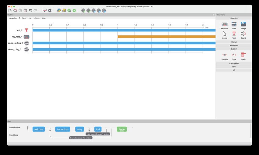
2. You will see the “info dialog,” as shown in Figure 3;
3. Enter your own initials in the participant field to run;
4. Set the lab section to either L101 (Tuesday) or L102 (Thursday);
5. Verify that the value 10 is in the repeats field. This number tells PsychoPy how many blocks of trials
to run under each orientation condition;
6. Click OK to begin the experiment.
Figure 3: The PsychoPy Information Dialog Box that pops up at the beginning of the experiment. The
information entered here will be included in the data file. Later you will learn how to add more information
if you need to.
Follow the on-screen instructions to do the experiment. Consider running a number of practice trials. After
4you feel comfortable with the task, abort the experiment by pressing the ‘esc’ key on the keyboard. Then
start the experiment again and follow it to completion. The program will run two blocks of 240 trials: one
block with the standard orientation set to 0 deg (vertical strips) and the other block with the standard
orientation set to 45 deg (oblique strips). It’s a lot of trials, so take occasional breaks.
On each trial you will first be presented with the standard stimulus (either 0 or 45 deg, depending on the
condition) followed by a test stimulus. The test will be rotated slightly counterclockwise or clockwise relative
to the standard. You must judge which by pressing the left arrow key (if you think the second stimulus is
counterclockwise) or the right arrow key (if you think it was clockwise). On each trial the computer will
record your responses. Some of the judgments will be easy and some will be difficult. The whole experiment
should not take more than 30 minutes. Figure 1 shows two examples of Gabor patches: the one on the left is
oriented at 0.0 degrees (vertical) and the other is tilted clockwise by 2.0 degrees. Can you see the difference?
Your experimental data will be saved automatically in the data folder in a text file whose name starts with
your initials with the date and time added to it. The file extension is csv (comma-separated values). After
the experiment has finished you can double click on the file to open in Excel. Do not edit or modify this
data file in any way. It represents a lot of judgments and work on your part. When you quit Excel do
not save the file if Excel asks you to.
Using a web browser, log onto Canvas at https://canvas.colorado.edu, and upload your data csv file to the
Lab 1 Data File dropbox in Assignments under Lab Individual Data Files (upload csv data files). If you
ran a practice run or two before running the proper experiment, only upload the final (latest) csv data file
to Canvas. This file will contain all your data. The other files are incomplete and don’t need to be saved.
But don’t delete anything to make sure you don’t accidentally delete a critical and irreplaceable file!
Next week, in Lab 2, you will analyze your individual data as well as the aggregated data from all the
students in the class. You will learn how to prepare a complete lab report and produce a finished, elegant,
pdf document.
5Lab 1 (Part 2): Data Analysis With
RStudio
Overview of Lab 1 Part 2
The goal of part 2 of this lab is to introduce several key features of RStudio (RStudio Team, 2021) that will
allow you to use it as a text processor with R Markdown and as an interface to R (R Core Team, 2021) for
making calculations and creating graphs. In this course your homework and lab reports will be submitted as
pdf files created by RStudio based on the principles of Open Science (https://en.wikipedia.org/wiki/Center_
for_Open_Science and https://opensciencetools.org). Today you will learn the basics. Next week you will
perform an experiment and learn how to create a complete lab report.
You will learn how to produce homework and lab reports using RStudio and R Markdown. R Markdown
provides a simple way to format text documents and include graphs and statistical analyses you do with R into
your final document. More information about R Markdown is found here: https://rmarkdown.rstudio.com.
You will also learn how to include citations to published research and to automatically generate a reference
section, as is done at the end of this document.
Goal 1: Organize
Each assignment or project must have its own RStudio project folder. That project folder will contain all
the files and data you need to produce your final document. You can save the folder to a flash drive or
compress it to a zip file and upload it to Google Drive or any other place to save it. Do not save it on the
lab computers: it will be gone after you log out.
Step 1: Download the Lab 1 Report Folder
1. In a web browser, navigate to the course webpage; http://psych.colorado.edu/~lharvey/P4165/P4165_
2021_3_Fall/Main_Page_2021_Fall_PSYC4165.html
2. Download the Lab_1_Report folder by clicking on the link Report Templates from the course main
page in the Lab Material section.
3. On the Mac the folder will be unzipped and be found in the Downloads folder;
4. If it is not unzipped, just double-click on it to get the folder;
5. Move the Lab_1_Project folder from Downloads into your master Lab 1 folder that is on your Desktop.
Step 2: Launch RStudio using the Project File
Launch RStudio by double clicking on the _Lab_1_Report.Rproj file inside the project folder. RStudio will
open a new window for the project with the working directory set to the project folder.
Step 3: Make a new R Markdown File
1. Select File > New File > R Markdown
2. Call the new file Lab 1: My First R Markdown
3. Enter your name in the name field
4. Click on the PDF radio button
65. Click OK and a new R Markdown document will appear in the RStudio editor in the upper left panel
of RStudio
6. Save the untitled document (it will be named Untitled1) with a name like lab1. RStudio will auto-
matically add the extension Rmd (R Markdown) to the file name to indicate that it is an R Markdown
document.
Edit the New R Markdown File
The first six lines of your file should look like this (replace the “??” with today’s date):
---
title: ’Lab 1: My First R Markdown’
author: "Your Name"
date: "31 August or 2 September 2021"
output: pdf_document
---
These lines at the top of your file, between the two --- lines, contain information that gives R Markdown
information about how to format the rest of your document. This information is called the YAML, YAML
metadata or YAML Header. Generally you don’t need to change it and you should not change it unless you
know what you are doing.
All the material that follows the YAML, after the second ---, is either R Markdown text that will be formatted
when you knit it or r code in code chunks that will be executed and whose output will be knitted into the
final document. Code chunks start with and end with three back ticks and appear shaded in gray. The first
code chunk is the setup chunk. In your file, select all the material below the setup code chunk and delete
it (from ## R Markdown to the end of the file.).
You will need to load a few additional R packages into your session. The usual way is to use the library()
command(s) and put them in the setup code chunk.
Add the two library commands shown below to the setup code chunk after the knitr line:
knitr::opts_chunk$set(echo = TRUE)
library("knitr")
library("tidyverse")
Goal 2: Read Data into R
In previous classes you learned how to attach data to your R code but we are going to use a much better
way to get data into R: by reading a file that contains the data and storing the data in an R data frame.
Step 2: Read Data into a Data Frame
Add a code chunk to your R Markdown script to read in the data using the read.csv() command. The
code chunk should look like this:
dfThese data were supplied by Caroline A. Davis, York University, for inclusion in the carData R package.
An example of her research is found here (Davis, 1990). I have edited the data set slightly to remove several
typographic errors in the original data. These data come from a large study of exercising men and women
and how they differ in the relationship between estimated body weight and height and actual weight and
height.
After being read into R the data frame df now holds six columns of height and weight data from 200 male
and female subjects. The six columns are subject, sex, weight, height, repwt (self-reported weight), and
repht (self-reported height).
These data are in a form called “tidy data” which is great for making graphs and doing statistical analyses.
Tidy data is a standard way of mapping the meaning of a dataset to its structure. A dataset is messy or
tidy depending on how rows, columns and tables are matched up with observations, variables and types. In
tidy data:
1. Each variable forms a column (e.g., subject, sex, weight, height, etc.)
2. Each observation forms a row. (e.g., measurements taken at one trial of an experiment)
3. Each type of observational unit forms a table. (e.g., all the rows and columns of each subject)
You will be happy to know that the csv data files produced by PsychoPy are tidy. Find out more about tidy
data here: https://tidyr.tidyverse.org/articles/tidy-data.html.
Goal 3: Graph the Data
We’ll make a scatter plot of height vs. weight for each of the 200 subjects using the ggplot package that is
part of the tidyverse set of packages. You must tell ggplot() three things in order to make a plot:
1. The name of the data frame that holds the data;
2. What aspects of the graph will be related to which data columns (the aesthetics);
3. What geometric representation will be used to plot the data (the geoms).
Here is a code chunk that will get you started. Add it to your R Markdown. We will show you how to make
the data appear, how to make better graph labels and how to add a figure legend.
ggplot(df, aes(x = weight, y = height))
Goal 4: Statistical Analysis
What kind of test would you use to see if sex influences height? We’ll show you how to do an ANOVA and
create tables of the results.
Goal 5: Create a pdf file and upload it to Canvas
You are now ready to produce a formatted pdf document that you will upload to the assignment section of
Canvas. Just click the Knit tab at the top left of the edit pane. RStudio will then knit your text and your
R code and its output together to create a pdf file for your enjoyment. Be sure to upload this pdf file to the
Assignment Lab 1 folder in Canvas.
8Save Your Lab 1 Master Folder
Make a zip archive of your Lab 1 master folder (control-click on the folder and select the Compress option)
and upload it to your Google Drive or other safe place. Once you log out of the lab computer all your work
will be lost after about 5 minutes!
Congratulations
You have been exposed to a lot of new material today. If you feel overwhelmed, hang in there. By the end
of the semester you will feel at home with all of this material as hard as this is to believe now. Andrew and
I are here to help you so ask questions when you don’t understand the material.
9Notes
Experiments in this course will be run using the PsychoPy program (Peirce, 2009, 2007; Peirce et al., 2019;
Peirce & MacAskill, 2018). PsychoPy is free, open-source software that runs on Macintosh, Windows and
Linux computers. Experiments built with PsychoPy can also be run online using the Pavlovia servers. Check
out the PsychoPy web site for more information: https://www.psychopy.org.
This document was prepared with RStudio (RStudio Team, 2021) using the R Markdown language. Sta-
tistical analyses, tables and graphs were produced with R [Version 4.1.1; R Core Team (2021)] and the
R-packages dplyr [Version 1.0.7; Wickham et al. (2021)], forcats [Version 0.5.1; Wickham (2021a)], ggplot2
[Version 3.3.5; Wickham (2016)], knitr [Version 1.33; Xie (2015)], papaja [Version 0.1.0.9997; Aust & Barth
(2020)], purrr [Version 0.3.4; Henry & Wickham (2020)], readr [Version 2.0.1; Wickham & Hester (2021)],
stringr [Version 1.4.0; Wickham (2019)], tibble [Version 3.1.4; Müller & Wickham (2021)], tidyr [Version
1.1.3; Wickham (2021b)], and tidyverse [Version 1.3.1; Wickham et al. (2019)].
10References
Appelle, S. (1972). Perception and discrimination as a function of stimulus orientation: The "oblique effect"
in man and animals. Psychological Bulletin, 78 (4), 266–278. https://doi.org/doi:10.1037/h0033117
Aust, F., & Barth, M. (2020). papaja: Create APA manuscripts with R Markdown. https://github.com/
crsh/papaja
Davis, C. (1990). Body image and weight preoccupation: A comparison between exercising and non-
exercising women. Appetite, 15 (1), 13–21. https://doi.org/10.1016/0195-6663(90)90096-Q
Fechner, G. T. (1860). Elemente der Psychophysik. Breitkopf and Härtel.
Freeman, J., Brouwer, G. J., Heeger, D. J., & Merriam, E. P. (2011). Orientation Decoding Depends on Maps,
Not Columns. The Journal of Neuroscience, 31 (13), 4792–4804. https://doi.org/10.1523/jneurosci.5160-
10.2011
Henry, L., & Wickham, H. (2020). Purrr: Functional programming tools. https://CRAN.R-project.org/
package=purrr
McMahon, M. J., & MacLeod, D. I. A. (2003). The origin of the oblique effect examined with pattern
adaptation and masking. Journal of Vision, 3 (3), 230–239. https://doi.org/10.1167/3.3.4
Meng, X., & Qian, N. (2005). The oblique effect depends on perceived, rather than physical, orientation and
direction. Vision Research, 45 (27), 3402–3413. https://doi.org/http://dx.doi.org/10.1016/j.visres.2005.
05.016
Müller, K., & Wickham, H. (2021). Tibble: Simple data frames. https://CRAN.R-project.org/package=
tibble
Nasr, S., & Tootell, R. B. H. (2012). A Cardinal Orientation Bias in Scene-Selective Visual Cortex. The
Journal of Neuroscience, 32 (43), 14921–14926. https://doi.org/10.1523/jneurosci.2036-12.2012
Peirce, J. W. (2009). Generating stimuli for neuroscience using PsychoPy. Frontiers in Neuroinformatics,
2 (January), 1–8. https://doi.org/10.3389/neuro.11.010.2008
Peirce, J. W. (2007). PsychoPy–Psychophysics software in Python. Journal of Neuroscience Methods,
162 (1-2), 8–13. https://doi.org/10.1016/j.jneumeth.2006.11.017
Peirce, J. W., Gray, J. R., Simpson, S., MacAskill, M., Höchenberger, R., Sogo, H., Kastman, E., & Lindeløv,
J. K. (2019). PsychoPy2: Experiments in behavior made easy. Behavior Research Methods, 51 (1), 195–
203. https://doi.org/10.3758/s13428-018-01193-y
Peirce, J. W., & MacAskill, M. (2018). Building Experiments in PsychoPy (1st edition.). SAGE Publications.
R Core Team. (2021). R: A language and environment for statistical computing. R Foundation for Statistical
Computing. https://www.R-project.org/
RStudio Team. (2021). RStudio: Integrated development environment for r. http://www.rstudio.com/
Westheimer, G. (2003). Meridional anisotropy in visual processing: Implications for the neural site of the
oblique effect. Vision Research, 43 (22), 2281–2289. https://doi.org/http://dx.doi.org/10.1016/S0042-
6989(03)00360-2
Wickham, H. (2016). ggplot2: Elegant graphics for data analysis. Springer-Verlag New York. https://
ggplot2.tidyverse.org
Wickham, H. (2019). Stringr: Simple, consistent wrappers for common string operations. https://CRAN.R-
project.org/package=stringr
Wickham, H. (2021a). Forcats: Tools for working with categorical variables (factors). https://CRAN.R-
project.org/package=forcats
Wickham, H. (2021b). Tidyr: Tidy messy data. https://CRAN.R-project.org/package=tidyr
11Wickham, H., Averick, M., Bryan, J., Chang, W., McGowan, L. D., François, R., Grolemund, G., Hayes,
A., Henry, L., Hester, J., Kuhn, M., Pedersen, T. L., Miller, E., Bache, S. M., Müller, K., Ooms, J.,
Robinson, D., Seidel, D. P., Spinu, V., . . . Yutani, H. (2019). Welcome to the tidyverse. Journal of Open
Source Software, 4 (43), 1686. https://doi.org/10.21105/joss.01686
Wickham, H., François, R., Henry, L., & Müller, K. (2021). Dplyr: A grammar of data manipulation.
https://CRAN.R-project.org/package=dplyr
Wickham, H., & Hester, J. (2021). Readr: Read rectangular text data. https://CRAN.R-project.org/
package=readr
Xie, Y. (2015). Dynamic documents with R and knitr (2nd ed.). Chapman; Hall/CRC. https://yihui.org/
knitr/
12You can also read