Study on a CNN-HMM Approach for Audio-Based Musical Chord Recognition - IOPscience

Journal of Physics: Conference Series

PAPER • OPEN ACCESS

Study on a CNN-HMM Approach for Audio-Based Musical Chord
Recognition
To cite this article: Taixiang Li 2021 J. Phys.: Conf. Ser. 1802 032033

View the article online for updates and enhancements.

 This content was downloaded from IP address 46.4.80.155 on 05/04/2021 at 09:38

CDMMS 2020 IOP Publishing
Journal of Physics: Conference Series 1802 (2021) 032033 doi:10.1088/1742-6596/1802/3/032033

Study on a CNN-HMM Approach for Audio-Based Musical
Chord Recognition

 Taixiang Li
 Longgang Intelligent Technology Co., Ltd, Changsha, 410016, China

 Taixiang@lgit.com.cn

 Abstract. Convolutional Neural Network (CNN) has shown its strength in image
 processing task, and Hidden Markov model (HMM) is a powerful tool for modeling
 sequential data. This paper presents a new architecture for audio-based chord
 recognition using a CNN-HMM mixture model. This architecture replaces the Gaussian
 mixture model (GMM) and Deep Neural Network (DNN) layers of GMM-HMM and
 DNN-HMM models with CNN. The model performance is evaluated through a dataset
 using different combinations of chroma vectors (STFT, CQT, CENS) as features, based
 on that, a scale recognition sub-model is tested.

 Keywords: Musical chord recognition; CNN; HMM; Chroma features; Musical scale
 recognition

1. Introduction
Music is widely held as an abstract theme of a particular art form that using sound to convey and elicit
emotion between players and listeners. It may be thought that music is just an unorganized subject that
expresses feelings through kinds of sound. However, music is not arbitrary, it follows specific rules.
Back to the 6 century BC, music has been analyzed in its most mathematical expression, called the
"Circle of Fifths", developed by Pythagoras. In the last few centuries, Fourier Transform (FT) presented
more analyzable features in the frequency domain. During the last decade, DNN has shown its strong
learning ability, and HMM has proved to be a powerful model for sequential data especially in
Automatic Speech Recognition (ASR) field [1]. Due to the sequential and frequency characteristics of
music (like speech), it is possible to analyze music in an ASR way.
 Musical chord is made up of at least three music notes, where notes with the same name from
different octaves are considered as one. In musical theory, a scale (key) is defined as a series of musical
notes arranged by the fundamental frequency. Due to the principle of octave equivalence, scales are
generally considered to span in a single octave. The whole frequency range is divided into 12 scales
(Minor scales are just relative scale of Major scales), and most of chords used in Western music are built
using the notes of a single scale. Besides, certain categories of music will only use certain chords in a
certain order for most of the piece, this order is called chord progression. Chord progression forms the
foundation of some of the most popular musical hits in modern music, some of them even sharing the
same progressions. Musical chord recognition is a fundamental problem in Music Information Retrieval
[2], its analysis is used in both classifying and generating new music pieces.

 Content from this work may be used under the terms of the Creative Commons Attribution 3.0 licence. Any further distribution
 of this work must maintain attribution to the author(s) and the title of the work, journal citation and DOI.
Published under licence by IOP Publishing Ltd 1

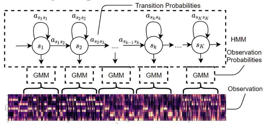
CDMMS 2020 IOP Publishing
Journal of Physics: Conference Series 1802 (2021) 032033 doi:10.1088/1742-6596/1802/3/032033

2. Background theory

2.1. Features: Chroma vectors
As shown by Muller [3], chroma-based audio features are suitable mid-level representations for
capturing musical information. Noted that the chroma features are based on the twelve-note attributes
 , #, . #, , , #, , #, , #, , where each element denotes the energy distribution across the 12
bands. Computing such distributions over time forms a time-frequency representation (chromagram),
thus making the chroma-based feature a suitable tool for chord recognition task.
 As the input audio is sequential, regular FT will not be considered as it abandons time-domain
information. Short-Time Fourier Transform (STFT) converts the time domain signal into an equivalent
mixed frequency-time domain signal by adding a window function to the FT. The definition is shown
below [4][5].

 [ , ] = ∑ [ ] ⋅ [ − ] ⋅ (1)

 However, STFT carries a constant bandwidth function, which leading to a problem that a larger
window size will result in higher spectral, but lower temporal resolution. And oppositely, a smaller size
will result in a lower spectral, but higher temporal resolution. Constant Q transform (CQT) with a
variable window size, luckily fixes this problem. The definition of CQT is listed below [5].

 [ ]
 [ ] = ∑ [ ] ⋅ [ , ] ⋅ [ ] (2)
 [ ]

 Besides, STFT chroma vectors after quantization and smoothing, called chroma energy normalized
statistics (CENS), are useful features for audio matching and similarity tasks. The main idea of CENS
is taking statistics over relatively large windows smooths out local deviations in tempo, articulation and
execution of note groups such as trills or arpeggios [3]. In this paper, we will compare and discuss the
performances of those three features in chord recognition tasks.

2.2. Traditional Acoustic Model
Similar to speech recognition, chord sequences are highly related to time. Markov Model (MM) can
partly fix the time correlation problem, assuming that the next state is only associated to its previous
with a particular transition probability. In practice, the Markov states are hidden beneath observation
states, these being the chroma vectors generated. Based on Markov chain, each state is equipped with a
probability function for a hidden state to an observation, called emission probability. The HMM
represents this connection using a probabilistic framework. The ideal chord sequence, in other words,
path with maximum probability, can be calculated optimally using the Viterbi algorithm as it is the best
solution to solve HMMs.
 As noted, musical chord recognition has similarities with speech recognition, the most general
method is via GMMs based HMMs (Figure 1), Bello and Pickens has shown the possibility of the GMM-
HMM model for solving chord recognition problem [6].

 Figure 1. GMM-HMM mixture model

 2

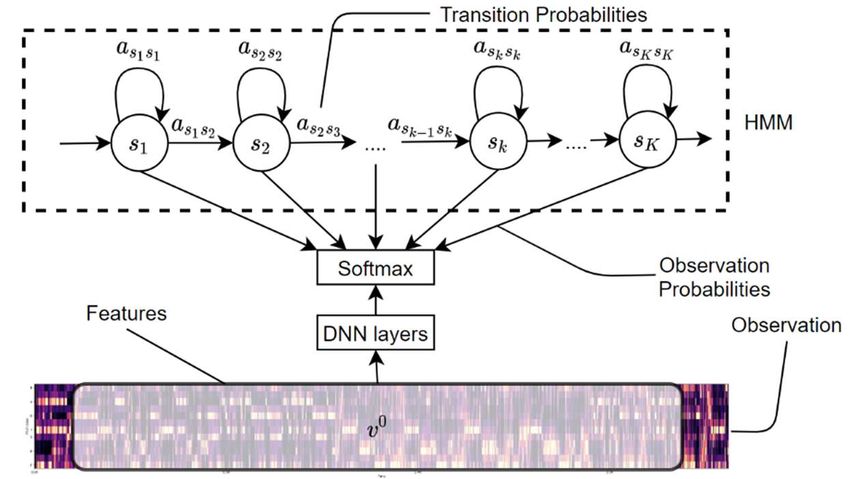
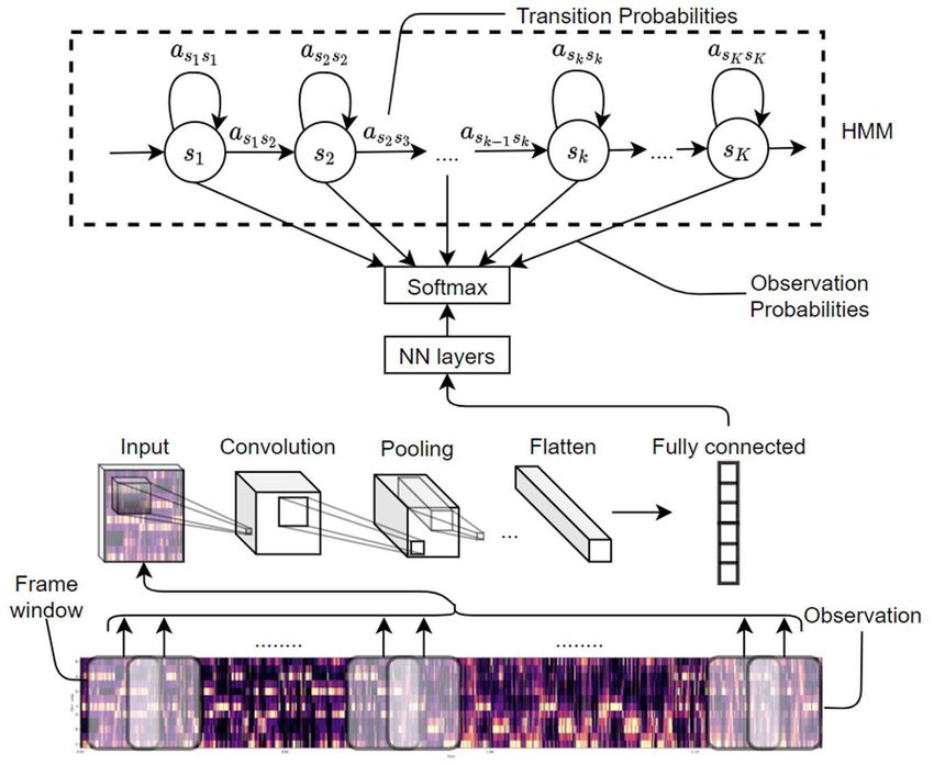
CDMMS 2020 IOP Publishing
Journal of Physics: Conference Series 1802 (2021) 032033 doi:10.1088/1742-6596/1802/3/032033

 Recently, DNN has shown its strong learning performance in classification tasks, however, it can not
be directly used in chord recognition tasks, as the input signal is sequential instead of constant sized.
The mixture model combining DNN and HMM (Figure 2) takes over the classification performance of
DNN, where HMM solves the sequential signal problem by using HMM to represent the dynamic
changes of the audio signal. Besides, using a frame window that contains all the information of the
adjacent frames can improve the performance of DNN-HMM model because DNN model somehow
mitigate the problem that HMM cannot satisfy the assumption of independence between states by
modeling the connections between different frames[1].

 Figure 2. DNN-HMM mixture model

3. Model Design

3.1. CNN-HMM
Based on DNN-HMM with a frame window, the input of DNN can be seen as a graph with size × ,
where is the number of features, and is the length of frame window. By transferring the
continuous audio model to a graphical model, CNN can be applied since it is the most appropriate model
in imaging processing. At this stage, the frame window can be expressed as a chord chromagram of that
moment, new features are extracted through convolution and pooling layers, which greatly simplified
the network structure. In Section 5, we compared the performances of GMM-HMM, DNN-HMM and
CNN-HMM in different conditions.

 3

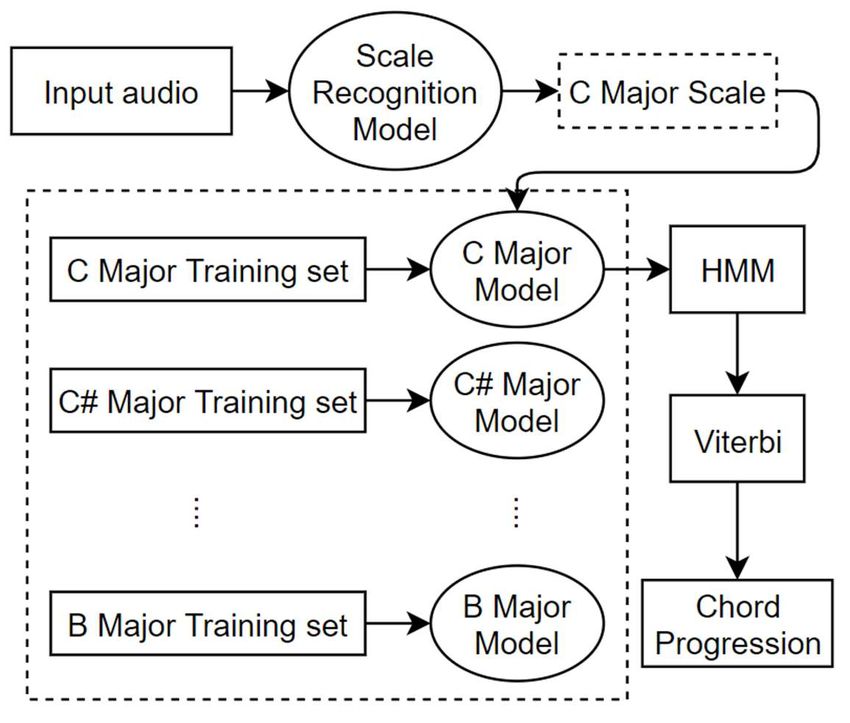
CDMMS 2020 IOP Publishing
Journal of Physics: Conference Series 1802 (2021) 032033 doi:10.1088/1742-6596/1802/3/032033

 Figure 3. CNN-HMM mixture model

3.2. Scale Recognition
Noted that a single piece of music is likely built using the notes of an individual scale, and the chords
used will be limited. Thus, the classification sets could be largely narrowed after identifying scales. On
the basis of knowing the scale, the classification performance can be improved, the CNN-HMM model
embedded with scale recognition is shown in Figure 4.

 Figure 4. Embedded with scale recognition (C Major Scale detected)

 4

CDMMS 2020 IOP Publishing
Journal of Physics: Conference Series 1802 (2021) 032033 doi:10.1088/1742-6596/1802/3/032033

4. Model Characterization

4.1. HMM Characters
Same as speech recognition, HMM used here is to find the most likely explanation of chord progressions.
Going back to Bayes' Rule:
 ⃗ ⃗ ⋅ ⃗
 ⃗ ⃗ = (3)
 ⃗

 The goal is to find the optimal chord sequence ⃗ maximize the probability based on the given
observations ⃗ (chroma sequence), the HMM characters (Initial Probability Matrix), (Transition
Probability Matrix) and (Emission Probability Matrix) are defined as following.

 (4)

 The first sample taken has no previous chord to rely on, thus matrix is assumed to have a uniform
distribution. The transition matrix can be calculated through whether training data or the nested
circle of fifths (based on music theory) [6], at this stage, we used the predefined nested circle of fifths
based version since the training data is not well-balanced.
 In GMM-HMM model, matrix is expressed as probability density function (pdf) values of a 12-
D multivariate Gaussian distribution (N=12) with certain mean and covariance matrices [6].

 P(O |μ, Σ) = (2π) ⋅ |Σ| ⋅ e
 ( ) ⋅ ⋅( ) (5)
 Since HMM needs likelihood probability ( | ), but the Softmax layer in DNN-HMM and CNN-
HMM only outputs a posterior probability, it needs to be transferred to likelihood probability through
Bayes:
 = ( ) = 
 ( | ) = = (6)
 ( ) ( )
 where = / is the prior probability obtained through the training data, is the number of
frames of state , and is the total number of frames [1]. ( ) is ignored because it is irrelevant
with chord sequence.

4.2. Window Size
As introduced in Section 2, adding a window can improve the performance of DNN-HMM model, also
it is a necessary precondition for CNN model. The size of the window decides the classification
performance also the length of processing time. A smaller size will lead to a faster processing speed but
lower performance. Oppositely, a larger size will cause higher performance but a time-consuming
system. The choice of an appropriate window size will be discussed in the following section.

4.3. Dataset
The primary training data includes over 3 hours' pure chords' audio generated by piano, acoustic guitar,
electric guitar and string band, where each instrument is played in 4 different playing techniques
(tempo\beats). Model performance is evaluated through over 60 minutes' hit songs (70% in C Major
Scale) of Beatles, Bruno Mars, Coldplay, etc. Those tracks are divided into a training (75%) and
validation split (25%), and the addition training set is added to the pre-trained model for optimizing
purpose.

 5

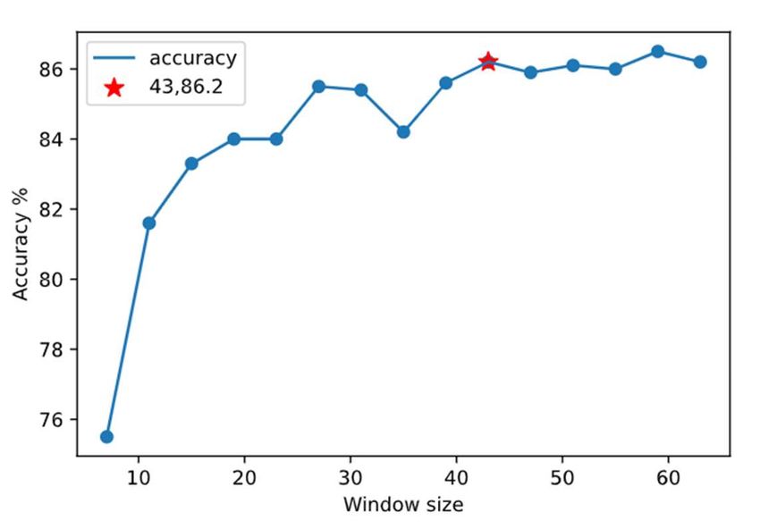
CDMMS 2020 IOP Publishing
Journal of Physics: Conference Series 1802 (2021) 032033 doi:10.1088/1742-6596/1802/3/032033

4.4. Network characters
The GMM model uses constant mean μ and covariance Σ matrices summarized from musical rules
[6]. The DNN and CNN models both have a Softmax output layer connected with several LeakyReLU
layers, and they both use Adam and categorical cross-entropy as their optimizer and loss function.
Besides, having a constant Dropout rate of 0.3 on all layers helps to reduce overfitting. We used a mini-
batch size of 256 and epochs of 20 for training. The DNN model was trained with three hidden layers
with varying number of units. While the CNN model was trained using two 2-D convolution-pooling
layers with convolution kernels of 4 × 4, connected with one hidden layer of 1920 units.
 Keep in mind that the output of the Softmax layer is not the final classification result, it was then be
transferred to emission probabilities by equation (6). The final chord progression is the output of HMM
through Viterbi algorithm.

5. Results
Because of the sequential property of chord progression, random splitting method k-fold validation
cannot be applied. Instead, a holdout validation was used. The following tables present the validation
results on the given dataset at 25 (24 chords plus one no chord zone) categories. The effect of scale
recognition and window size is evaluated by the CNN-HMM model with STFT&CQT&CENS as
features.

5.1. Chroma features and Models

 Table 1. Validation results of features and models (window size = 43)
 Model (~HMM)
 Feature
 GMM DNN CNN
 STFT 38.3% 61.5% 75.3%
 CQT 52.4% 65.0% 84.2%
 CENS 29.7% 78.2% 80.8%
 STFT&CQT None 82.5% 83.0%
 STFT&CENS None 75.7% 85.8%
 CQT&CENS None 60.7% 84.7%
 STFT&CQT&CENS None 84.9% 86.5%

 Table 1 shows the outcomes of different chroma features in various models. It is clear that
introducing more features improves the performance of DNN-HMM and CNN-HMM models, while the
CNN-HMM performs better (around 1.5% ahead). Since the dataset is limited to a small size, the
performance of unsupervised learning GMM is limited, noted that the multiple combination of chroma
vectors for GMM were not tested due to the uncertainty of covariance matrix [6].

5.2. Scale recognition

 Table 2. Validation results of SR (Scale recognition) in different scales (window size = 43)
 Scale
 Model
 C Major E Major A Major
 With SR 89.8% 84.5% 79.3%
 Without SR 89.5% 82.3% 77.2%

 6

CDMMS 2020 IOP Publishing
Journal of Physics: Conference Series 1802 (2021) 032033 doi:10.1088/1742-6596/1802/3/032033

 Noted that around 70% of the training songs are in C Major scale, thus the model trained is mostly a
model suits C Major song. As shown in Table 2, the accuracy of C Major songs roughly stays constant,
but songs in other scales have an increment of 2% in accuracy. It indicates that the scale recognition will
correct the model when the training data is not well-balanced.

5.3. Window size

 Figure 5. CNN-HMM with varying window size

 As outlined before, adding a frame window will help to strengthen the ability to process sequential
data. There is a trade-off when choosing the window size. Figure 5 shows the performance of the CNN-
HMM model with various window sizes. The accuracy increases with growing window size, and it
roughly stopped when window size number reached 43, where gives an accuracy of 86.2%. Based on
that, the recommended window size for this sampling rate is 43.

6. Conclusion and Future work
This paper presents a CNN-HMM approach to solve chord recognition task. Through the analysis of
different chroma features, using a combination of STFT&CQT&CENS can largely improve the
performance. Besides, embedding a scale recognition model can fix the training data balancing issue to
a certain extent. A suitable frame window size helps to model the sequential feature, also it is a necessary
condition for transferring DNN to a CNN model.
 This small dataset will not cover features for multiple music types such as Pop, Jazz, Blues, R&B,
etc., using a comprehensive dataset or modeling based on music type will enlarge the performance for
music with different styles. Also, considering the complexity of modeling, we only focused on songs
within the 24 basic chords. However, each of the basic chord has a series of sub-chords such as Aug,
Dim, Maj7, etc., building such a model that covers all the chords will help to present the diversity of
music.

Acknowledgements
This research was inspired by Prof. Margreta Kuijper. I wish to thank Prof. Quangui Wang for his
insightful comments and careful reading of the script.

 7

CDMMS 2020 IOP Publishing
Journal of Physics: Conference Series 1802 (2021) 032033 doi:10.1088/1742-6596/1802/3/032033

References
[1] Dong Yu, Li Deng. Automatic Speech Recognition: A Deep Learning Approach. 2015, p. 1-116.
[2] Matt McVicar, Raúl Santos-Rodríguez, Yizhao Ni, Tijl De Bie. Automatic Chord Estimation from
 Audio: A Review of the State of the Art. IEEE/ACM Transactions on Audio, Speech, and
 Language Processing, 22(2):556–575, 2014.
[3] Meinard Müller. Fundamentals of Music Processing. 2015, p. 1-300.
[4] Judith. C. Brown. Calculation of a constant Q spectral transform. The Journal of the Acoustical
 Society of America, vol. 89 (1991), no. 1, p. 425-434.
[5] Shibli Nisar, Omar Usman Khan, Muhammad Tariq. An Efficient Adaptive Window Size Selection
 Method for Improving Spectrogram Visualization. 2016.
[6] Bello, J., Pickens, J. A Robust Mid-level Representation for Harmonic Content in Music Signals.
 2005.

 8