Superior Predictability of American Factors of the Won/Dollar Real Exchange Rate
←
→
Page content transcription
If your browser does not render page correctly, please read the page content below
Auburn University
    Department of Economics
    Working Paper Series

Superior Predictability of American
Factors of the Won/Dollar Real
Exchange Rate
Sarthak Behera*, Hyeongwoo Kim†, and Soohyon Kim‡

Centre College, †Auburn University, ‡Chonnam
*

National University

AUWP 2021‐03

This paper can be downloaded without charge from:

    http://cla.auburn.edu/econwp/

    http://econpapers.repec.org/paper/abnwpaper/
Superior Predictability of American Factors of the
        Won/Dollar Real Exchange Rate
           Sarthak Beheray, Hyeongwoo Kimz, and Soohyon Kimx

                                        July 2021

                                         Abstract

         Utilizing an array of data dimensionality reduction methods, we estimate
      latent common factors of the Won/Dollar real exchange rate from a large panel
      of economic predictors of the U.S. and South Korea. We demonstrate supe-
      rior out-of-sample predictability of our factor augmented forecasting models
      relative to conventional models when we utilize factors obtained from U.S.
      economic variables, while Korean factors fail to enhance predictability. Our
      models perform better at longer horizons when American real activity factors
      are employed, whereas American nominal/…nancial market factors help im-
      prove short-run prediction accuracy. UIP fundamental factors with the dollar
      as numéraire overall perform well, while PPP and RIRP factors play a limited
      role in forecasting the Won/Dollar exchange rate.

      Keywords: Won/Dollar Real Exchange Rate; Principal Component Analysis;
      Partial Least Squares; LASSO; Out-of-Sample Forecast

      JEL Classi…cation: C38; C53; C55; F31; G17

     We thank seminar participants at the Bank of Korea for useful comments.
  y
     Economics and Finance Program, Centre College, 319 Crounse Hall, Danville, KY 40422. Tel:
+1-859-238-5235. Email: sarthak.behera@centre.edu.
   z
     Department of Economics, Auburn University, 138 Miller Hall, Auburn, AL 36849. Tel: +1-
334-844-2928. Fax: +1-334-844-4615. Email: gmmkim@gmail.com.
   x
     Chonnam National University, 77, Yongbong-ro, Buk-gu, Gwangju, 61186, Korea, Tel: +82-62-
530-1540, Email: soohyon.kim@jnu.ac.kr.

                                              1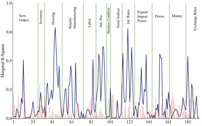
1       Introduction
This paper presents factor-augmented forecasting models for the real exchange rate
between Korea and the U.S. We demonstrate superior out-of-sample prediction per-
formance of our models over commonly used benchmark models when we employ
latent factors that are extracted from a large panel of macroeconomic time series
data in the U.S. On the other hand, we report a very limited role of factors from
Korean macroeconomic variables in predicting the real exchange rate. We interpret
such superb forecastability exclusive to American factors as a consequence of high
degree of cross-correlations between bilateral real exchange rates vis-à-vis the U.S.
dollar.
    In their seminal work, Meese and Rogo¤ (1983) demonstrate that the random
walk (RW) model performs well in forecasting exchange rates in comparison with the
models that are motivated by exchange rate determination theories. Cheung, Chinn,
and Pascual (2005) add more evidence of such a disconnect between the exchange
rate and economic fundamentals, showing that exchange rate models still do not
consistently outperform the RW model in out-of-sample forecasting.1 In a related
work, Engel and West (2005) provide an interesting point that asset prices such as
the exchange rate can show a near unit root process, though these prices are still
consistent with asset pricing models as the discount factor approaches one.2
    However, a group of researchers demonstrated that exchange rate models could
outperform the RW model at longer horizons. For example, Mark (1995) used a re-
gression model of multiple-period changes (long-di¤erenced) in the nominal exchange
rate on the deviation of the exchange rate from its fundamentals, then reported over-
all superior long-horizon predictability of fundamentals for the exchange rate. Chinn
and Meese (1995) also report similar long-horizon evidence of greater predictability
of exchange rate models relative to the RW. Using over two century-long annual fre-
quency data, Lothian and Taylor (1996) report good out-of-sample predictability of
fundamentals for the real exchange rate. Groen (2005) reports some long-horizon
evidence of superior predictability of monetary fundamentals employing a vector au-
toregressive (VAR) model framework.3 Also, Engel, Mark, and West (2008) show
    1
     However, Engel and Hamilton (1990) report some evidence that their nonlinear models outper-
form the RW. But their …ndings are still at odds with uncovered interest parity (UIP).
   2
     Many researchers provide panel evidence of a close link between monetary models and exchange
rate dynamics. See for example, Rapach and Wohar (2004), Groen (2000), and Mark and Sul (2001).
   3
     They demonstrate that the monetary fundamentals-based common long-run model tends to
outperform the RW model as well as the standard cointegrated vector autoregressive (VAR) model

                                               2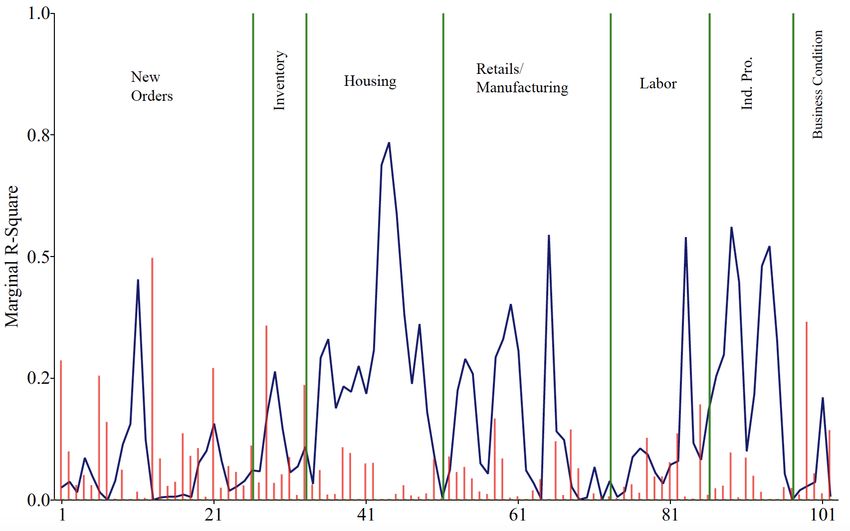
that out-of-sample predictability can be enhanced by focusing on panel estimation
and long-horizon forecasts.
    Another group of researchers started using Taylor Rule fundamentals in addition
to conventional monetary fundamentals. See among others, Engel, Mark, and West
(2008), Molodtsova, Nikolsko-Rzhevskyy, and Papell (2008), Molodtsova and Papell
(2009), Molodtsova and Papell (2013), and Ince, Molodtsova, and Papell (2016). They
show that models with Taylor Rule fundamentals tend to perform well in forecasting
the exchange rate. See Rossi (2013) for a survey of research work that demonstrates
the importance of Taylor Rule fundamentals in understanding exchange rate dynam-
ics.4
    We note that the pioneering work of Stock and Watson (2002) has initiated an
in‡ux of papers that utilize latent common factors in forecasting macroeconomic vari-
ables via principal components (PC) analysis. The current exchange rate literature
is not an exception. A number of researchers began using large panels of time se-
ries data to better understand exchange rate dynamics. For instance, Engel, Mark,
and West (2015) use cross-section information (PC factors) that are obtained from a
panel of 17 bilateral exchange rates relative to the US dollar, then demonstrate that
factor based forecasting models often outperform the RW model during the post-1999
sample period. They also report good forecasting performance of the dollar factor
in combination with Purchasing Power Parity (PPP) factors. Chen, Jackson, Kim,
and Resiandini (2014) used PC to extract latent common factors from 50 world com-
modity prices. Their …rst common factor turns out to be closely related with the
dollar exchange rate, which is consistent with an observation that world commodities
are priced in U.S. dollars. They show that this …rst common factor yields superior
out-of-sample predictive contents for the dollar exchange rate.
    Greenaway-McGrevy, Mark, Sul, and Wu (2018) demonstrate that exchange rates
are mainly driven by a dollar and an euro factor. They show that their dollar-euro
factor model dominates the RW model in the out-of-sample prediction performance.
Verdelhan (2018) uses portfolios of international currencies to extract the two risk fac-
tors (dollar factor and carry factor), which successfully explain exchange rate dynam-
at 2 to 4 year horizons.
   4
     In a related work, Wang and Wu (2012) show the superior out-of-sample interval predictability of
the Taylor Rule fundamentals at longer horizons. Also, many researchers report in-sample evidence
that Taylor rule fundamentals help understanding exchange rate dynamics. See among others, Mark
(2009), Molodtsova, Nikolsko-Rzhevskyy, and Papell (2008), Engel and West (2006), and Clarida
and Waldman (2008).

                                                 3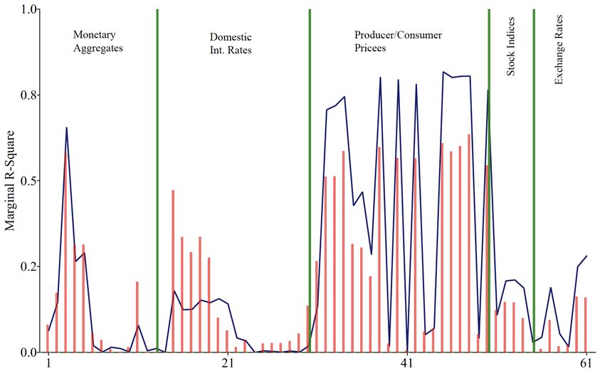
ics. Ca’Zorzi, Kociecki, and Rubaszek (2015) demonstrate that structural Bayesian
vector autoregression (SBVAR) models with a Dornbusch prior tend to outperform
the RW model at medium horizons, although it is still di¢ cult to beat the RW model
in the short-run.
    PC has been widely used in the current forecasting and empirical macroeconomics
literature. However, it extracts latent common factors from predictors without con-
sidering the relationship between predictors and the target variable. As shown by
Boivin and Ng (2006), its performance may be poor in forecasting the target vari-
able if useful predictive contents are in a certain factor that is dominated by other
factors. Recognizing this potential problem, we employ an alternative data dimen-
sionality reduction method such as the partial least squares (PLS) method proposed
by Wold (1982). This method utilizes the covariance between the target and predictor
variables to generate target-speci…c factors. See Kelly and Pruitt (2015) and Groen
and Kapetanios (2016) for some comparisons between the PC and PLS approaches.
Similar to Bai and Ng (2008) and Kelly and Pruitt (2015), we also use the Least Ab-
solute Shrinkage and Selection Operator (LASSO) to select target-speci…c groups of
the predictors among the full dataset to extract more relevant factors for the target.
    In this paper, we suggest factor-augmented forecasting models for the KRW/USD
real exchange rate. We employ PC and PLS as well as the LASSO in combination
with PC and PLS to estimate common factors using large panels of 125 American and
192 Korean monthly frequency macroeconomic time series data from October 2000 to
March 2019. Since most macroeconomic data are better approximated by a nonsta-
tionary integrated process (Nelson and Plosser, 1982), we extract common factors by
applying these methods to …rst di¤erenced predictors to consistently estimate factors
(Bai and Ng, 2004). We also extract common factors from country-level global data
using up to 43 country-level data for prices and interest rates, motivated by exchange
rate determination theories such as Purchasing Power Parity (PPP), Uncovered In-
terest Parity (UIP), and Real Uncovered Interest Parity (RIRP). We then implement
an array of out-of-sample forecasting exercises utilizing these factor estimates, and
investigate what factors help improve the prediction accuracy for the exchange rate.
We evaluate the out-of-sample predictability of our factor models via the ratio of the
root mean squared prediction error (RRMSPE) criteria.
    Our major …ndings are as follows. First, our factor-augmented forecasting models
outperform the random walk (RW) and autoregressive AR(1) type benchmark models
only when they utilize American factors. Korean factor-augmented models overall got

                                          4
dominated by the AR model, although they still outperform the RW model when the
forecast horizon is one-year or longer. It is well known that bilateral exchange rates
relative to the U.S. dollar tend to exhibit high cross-correlations. That is, U.S. com-
mon factors are likely to dominate dynamics of these exchange rates vis-à-vis dollars
over idiosyncratic components in each country such as Korea. Combining Korean
(idiosyncratic) factors with American factors slightly improves the forecasting perfor-
mance but failed to observe su¢ ciently large improvement enough to outperform the
AR model.
    Second, our models tend to perform better in short horizons when they are com-
bined with nominal/…nancial market factors in the U.S. On the other hand, American
real activity factor models outperform both the RW and AR models at longer hori-
zons. Put it di¤erently, good short-run prediction performance of our models with the
total factors seems to inherit the superior performance of our models with …nancial
market factors, while superior long-run predictability seems to stem from information
from real activity factors. These results are consistent with the work of Boivin and
Ng (2006) in the sense that one may extract more useful information from subsets of
predictors.
    Third, forecasting models with UIP motivated factors perform well when the U.S.
serves as the reference country. However, PPP and RIRP based factor models are
dominated by the AR model whichever country serves as the reference. Overall,
data-driven factor models seem to perform better than these propositon-based factor
models.
    The rest of the paper is organized as follows. Section 2 carefully describes how
we estimate latent common factors via PC, PLS, and the LASSO for the real ex-
change rate when predictors obey an integrated process. Section 3 presents data
descriptions and preliminary statistical analysis. We also report some in-sample …t
analysis to investigate the source of latent common factors. In Section 4, we introduce
our factor-augmented forecasting models and evaluation schemes. Then, we present
and interpret our out-of-sample forecasting exercise results. We also report results
with alternative identi…cation approaches, proposition-based models and nonstation-
ary forecasting models, in comparison with the data-driven factor forecasting models.
Section 5 concludes.

                                          5
2 Methods of Estimating Latent Common Factors
This section explains how we estimate latent common factors by applying Principal
Component (PC), Partial Least Squares (PLS), and the Least Absolute Shrinkage
and Selection Operator (LASSO) to a large panel of nonstationary predictors.
2.1 Principal Component Factors
Since the seminal work of Stock and Watson (2002), PC has been popularly used in the
current forecasting literature. We begin with this approach to show how to estimate
latent common factors when predictors are likely to be integrated I(1) processes
largely based on the work of Bai and Ng (2004).
Consider a panel of N macroeconomic T 1 time series predictors/variables,
0
x = [x1 ; x2 ; :::; xN ], where xi = [xi;1 ; xi;2 ; :::; xi;T ] ; i = 1; :::; N . We assume that each
predictor xi has the following factor structure. Abstracting from deterministic terms,
0
PC
xi;t = i ft + "i;t ; (1)
0
PC PC PC
where ft = f1;t ; f2;t ; ; fR;t is an R 1 vector of latent time-varying common
0
factors at time t and i = [ i;1 ; i;2 ; ; i;R ] denotes an R 1 vector of time-invariant
idiosyncratic factor loading coe¢ cients for xi . "i;t is the idiosyncratic error term.
Following Bai and Ng (2004), we estimate latent common factors by applying
the PC method to …rst-di¤erenced data. This is because, as shown by Nelson and
Plosser (1982), most macroeconomic time series variables are better approximated
by an integrated nonstationary stochastic process. Note that the PC estimator of ft
would be inconsistent if "i;t is an integrated process. First di¤erencing (1), we obtain
the following.
0
xi;t = i ftP C + "i;t (2)
for t = 2; ; T . We …rst normalize the data, x ~ = [ x ~1 ; x ~N ], then
~2 ; :::; x
0
apply PC to x ~ x ~ to obtain the factor estimates ^ P C
ft along with their associated
factor loading coe¢ cients ^ i .5 Naturally, estimates of the idiosyncratic component
0
are obtained by taking the residual, ^"i;t = x~i;t ^i ^ftP C . The level variable
5
This is because PC is not scale invariant. We demean and standardize each time series.
6estimates are recovered via cumulative summation as follows.
X
t X
t
^"i;t = ^"i;s ; ^
ftP C = ^
fsP C (3)
s=2 s=2
It should be noted that this procedure yields consistent factor estimates even when
x includes some stationary I(0) variables. For example, assume that xj , j 2 f1; :::; N g
is I(0). Di¤erencing it once results in xj , which is still stationary, I( 1). Therefore
the PC estimator remains consistent. Alternatively, one may continue to di¤erence
the variables until the null of nonstationarity hypothesis is rejected via a unit root
test.6 However, this may not be practically useful when unit root tests provides
contradicting statistical inferences under alternative test speci…cations (i.e., number
of lags, number of observations). See Cheung and Lai (1995) for related discussions.
2.2 Partial Least Squares Factors
We employ PLS for a scalar target variable qt , which is somewhat overlooked in the
current literature. Unlike PC, the method of PLS generates target speci…c latent
common factors, which is an attractive feature. As Boivin and Ng (2006) pointed
out, PC factors might not be useful in forecasting the target when useful predictive
contents are in a certain factor that may be dominated by other factors.
PLS is motivated by the following linear regression model. Abstracting from
deterministic terms,
0
q t = xt + e t ; (4)
where xt = [ x1;t ; x2;t ; :::; xN;t ]0 is an N 1 vector of predictor variables at time
t = 1; :::; T , while is an N 1 vector of coe¢ cients. et is an error term. Again, we
…rst-di¤erence the predictor variables assuming that xt is a vector of I(1) variables..
PLS is especially useful for regression models that have many predictors, when N
is large. To reduce the dimensionality, rewrite (4) as follows,
0
qt = xt w + u t (5)
P LS 0
= ft + ut
0
where ftP LS = P LS
f1;t P LS
; f2;t P LS
; :::; fR;t ; R < N is an R 1 vector of PLS
6
This approach is used to construct the Fred-MD database. The Fred-MD is available at
https://research.stlouisfed.org/econ/mccracken/fred-databases/.
7factors. Note that ftP LS is a linear combination of all predictor variables, that is,
0
ftP LS = w xt ; (6)
0
where w = [w1 ; w2 ; :::; wR ] is an N R weighting matrix. That is, wr = [w1;r ; w2;r ; :::; wN;r ] ,
r = 1; :::; R, is an N 1 vector of weights on predictor variables for the rth PLS factor,
P LS
fr;t . is an R 1 vector of PLS regression coe¢ cients. PLS regression minimizes
the sum of squared residuals from the equation (5) for instead of in (4). It should
be noted that we do not utilize for our out-of-sample forecasting exercises in the
present paper. To make it comparable to PC factors, we utilize PLS factors ftP LS ,
then augment the benchmark forecasting model with estimated PLS factors ^ ftP LS .
Among available PLS algorithms, see Andersson (2009) for a brief survey, we use
the one proposed by Helland (1990) that is intuitively appealing. Helland’s algorithm
to estimate PLS factors for a scalar target variable qt is as follows. First, f^1;t P LS
is
pinned down by the linear combinations of the predictors in xt .
X
N
f^1;t
P LS
= wi;1 xi;t ; (7)
i=1
where the loading (weight) wi;1 is given by Cov(qt ; xi;t ). Second, we regress qt and
xi;t on f^1;t
P LS
then get residuals, q~t and x~i;t , respectively, to remove the explained
component by the …rst factor f^1;t P LS
. Next, the second factor estimate f^2;t P LS
is
obtained similarly as in (7) with wi;2 = Cov(~ qt ; x~i;t ). We repeat until the Rth factor
f^R;t
P LS
is obtained. Note that this algorithm generates mutually orthogonal factors.
2.3 Least Absolute Shrinkage and Selection Operator Factors
We employ a shrinkage and selection method for linear regression models, the LASSO,
which is often used for sparse regression. Unlike ridge regression, the LASSO selects a
subset (xs ) of predictor variables from x by assigning 0 coe¢ cient to the variables that
are relatively less important in explaining the target variable. Putting it di¤erently,
we implement the feature selection task using the LASSO.
The LASSO puts a cap on the size of the estimated coe¢ cients for the ordinary
least squares (LS) driving the coe¢ cient down to zero for some predictors. The
LASSO solves the following constrained minimization problem using L1 -norm penalty
on .
8( )
1X X
T N
0 2
min (qt xt ) ; s.t. j jj (8)
T t=1 j=1
where xt = [ x1;t ; x2;t ; :::; xN;t ]0 is an N 1 vector of predictor variables at time
t = 1; :::; T , is an N 1 vector of associated coe¢ cients. As the value of tuning
(penalty) parameter decreases, the LASSO returns a smaller subset of x, setting
more coe¢ cients to zero.
Following Kelly and Pruitt (2015), we choose the value of to generate a certain
number of predictors by applying the LASSO to x. We then employ the PC and
P C=L P LS=L
PLS approach to extract common factors, ft or ft , out of the predictor
variables that are chosen by the LASSO regression. Similar to our PLS approach,
we use the LASSO method only to obtain the subset of predictors that are closely
related to the target.
3 In-Sample Analysis
3.1 Data Descriptions
We obtained a large panel of 126 American macroeconomic time series variables from
the FRED-MD database. We also obtained 192 Korean macroeconomic time series
data from the Bank of Korea. Korea has maintained a largely …xed exchange rate
regime for the dollar-won exchange rate until around 1980, then switched to a heavily
managed ‡oating exchange rate regime. Korea continued dirty ‡oat or managed ‡oat
until they were forced to adopt a market based exchange rate regime after they got
hit by the Asian Financial Crisis in 1997.
We focus on the free ‡oating exchange rate regime in 2000’s after the Korean econ-
omy fully recovered from the crisis. Observations are monthly and span from October
2000 to March 2019 to utilize reasonably many monthly predictors in Korea. We use
the consumer price index (CPI) to transform the nominal KRW/USD exchange rate
to the real exchange rate.
We categorized 192 Korean predictors into 13 groups. Groups #1 through #6
include real activity variables that include inventories and industrial productions,
while groups #7 to #13 are nominal/…nancial market variables such as interest rates
and prices. See Table 1 for more detailed information. Similarly, we categorized 126
American predictors into 9 groups of variables. Groups #1 through #4 represent the
9real activity variables, while groups #5 through #9 are considered as …nancial sector
variable groups in the US. We log-transformed all quantity variables prior to estima-
tions other than those expressed in percent (e.g., interest rates and unemployment
rates).
Table 1 around here
3.2 Unit Root Tests
We …rst implement some speci…cation tests for our analysis. Table 2 presents the
augmented Dickey Fuller (ADF) test results for the log real exchange rate (qt =
st + pUt S pKR
t ) and the log nominal exchange rate (st ). The ADF test rejects the null
of nonstationarity for qt at the 5% signi…cance level, while it fails to reject the null
hypothesis for st at any conventional level. Note that these results are consistent with
standard monetary models in international macroeconomics. Recall, for example, that
purchasing power parity (PPP) is consistent with stationary qt and nonstationary st ,
because PPP implies a cointegrating relationship [1; 1] between st and the relative
price (relpt = pUt S pKRt ) for the real exchange rate qt in the long-run.
Next, we implement a panel unit root test for predictor variables in the US (xUt S )
and in Korea (xKR t ) via the Panel Analysis of Nonstationarity in Idiosyncratic and
Common components (PANIC) analysis by Bai and Ng (2004). The PANIC procedure
PC
estimates common factors (fr;t ; r = 1; 2; ::; R) via PC as explained in the previous
section, then test the null of nonstationarity for common factors via the ADF test with
an intercept. It also implements a panel unit root test for de-factored idiosyncratic
components of the data by the following statistic.
PN
2 ln pe^i
i=1 2N
Pe^ = ;
2N 1=2
where pe^i denotes the p-value of the ADF statistic with no deterministic terms for
de-factored xi;t .7
Note that we also test the null hypothesis for the common factors of subsets of xt ,
that is, real and …nancial sector variables separately. This is because we are interested
7
Pe^ statistic has an asymptotic standard normal distribution. The panel test utilizes the p-
value of the ADF statistics with no deterministic terms, because de-factored variables are mean-zero
residuals.
10in the out-of-sample predictability of the common factors from these subsets of the
P C;R
data. In what follows, we show American real activity factors (fr;t ; r = 1; 2; ::; R)
include more long-run predictive contents, whereas American …nancial market factors
P C;F
(fr;t ; r = 1; 2; ::; R) yield superior predictability in the short-run, which is consistent
with the implications of Boivin and Ng (2006).
The PANIC test fails to reject the null of nonstationarity for all common factor
estimates at the 5% signi…cance level with an exception of the second …nancial factor
in the US. Its panel unit root test rejects the null hypothesis that states all variables
are I(1) processes for all cases.8 However, nonstationary common factors eventually
dominate stationary dynamics of de-factored idiosyncratic components. Hence, test
results in Table 2 provide strong evidence in favor of nonstationarity in the predictor
variables xt , which is consistent with Nelson and Plosser (1982).
Table 2 around here
3.3 Factor Model In-Sample Analysis
This section describes some in-sample properties of the factor estimates we discussed
in previous section. Figure 1 presents in-sample …t analysis for the KRW/USD real
exchange rate. Three …gures in top row report cumulative R2 statistics of PC and
PLS factors obtained from all predictors, real activity predictors, and …nancial sector
predictors in the US, respectively from left to right. Three …gures in bottom row
provide cumulative R2 values of Korean factors similarly. Some interesting …ndings
are as follows.
First, the PLS factors (dashed lines) provide a notably better in-sample …t in
comparison with the performance of PC factors (solid lines). This is because PLS
utilizes the covariance between the target and the predictor variables, while PC fac-
tors are extracted from the predictor variables only. It is also interesting to see that
the cumulative R2 statistics of PLS factors overall exhibit a positive slope at a de-
creasing rate as the number of factors increases, whereas additional contributions
of PC factors show no such patterns. This is mainly due to the fact that our PLS
algorithm sequentially estimates orthogonalized common factors after removing ex-
planatory power of previously estimated factors. The PC method extracts common
8
The alternative hypothesis is that there is at least one stationary variable.
11factors without considering the target variable, hence the additional contribution of
PC factors does not necessarily decrease.
Second, American factors greatly outperform Korean factors. Cumulative R2
values of American PLS factors reach well above 60%, while Korean PLS factors
cumulatively explain less than 40% of variations in the real exchange rate. Note
that Korean PC factors yield virtually no explanatory power. These …ndings imply
that Korean macroeconomic variables might not play an important role in explain-
ing the Won/Dollar real exchange rate dynamics, while American predictors contain
substantial predictive contents for it.
We relate such …ndings with a strong degree of cross-correlations of many bilateral
exchange rates relative to the US dollars, implying that American factors better
explain dynamics of exchange rates vis-à-vis U.S. dollar than idiosyncratic factors in
local countries such as Korea. To see this, we implement a formal test by Pesaran
(2021) for the cross-section dependence in 36 bilateral real exchange rates against the
U.S. dollar including 16 eurozone countries.9 Consider the following test statistic.
s !
2T X1
N X
N
CD = ^i;j !d N (0; 1)
N (N 1) i=1 j=i+1
where ^i;j is the pair-wise correlation coe¢ cients from the residuals of the ADF re-
gressions for each real exchange rate.10 The CD statistic was 176:748 (pv = 0:000)
implying strong empirical evidence of cross-section dependence at any conventional
signi…cance level. The average ^i;j was 0:481. We obtained similar results even when
we exclude all eurozone countries. The CD statistic was 59:019 (pv = 0:000) and the
average ^i;j was 0:293. Such strong cross-correlations of many bilateral real exchange
rates imply a dominant role of the reference country, that is, the U.S. in determining
the dynamics of these bilateral exchange rates.
Third, PLS factors from American real activity groups and …nancial variable
9
We obtained all nominal exchange rates and CPIs from the IFS for the sample period from
September 2000 to December 2018. 16 eurozone countries that are included are Austria, Belgium,
Finland, France, Germany, Greece, Ireland, Italy, Latvia, Lithuania, Luxembourg, Netherlands,
Portugal, Slovakia, Slovenia, and Spain. We were able to retrieve 20 non-eurozone countries including
Brazil, Canada, Chile, China, Colombia, Czech Republic, Denmark, Hungary, India, Indonesia,
Israel, Japan, Korea, Mexico, Poland, Russia, Singapore, Switzerland, Sweden, and the UK. We
obtained the Singapore CPI from the Department of Statistics of Singapore.
10
We implemented the ADF regression for each real exchange rate relative to the U.S. dollar via
the general-to-speci…c rule with maximum 6 lags, then calculated pair-wise correlation coe¢ cients
using the ADF regression residuals of 35 real exchange rates.
12groups explain variations in the KRW/USD real exchange rate similarly well. On
the other hand, the contribution of PLS Korean factors mostly stem from that of
PLS Korean …nancial sector factors. PLS real Korean factors explain less than 10%
of variations jointly even when 12 factors are utilized.
Figure 1 around here
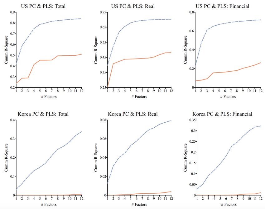
Next, we investigate the source of these common factor estimates via the marginal
R2 analysis. That is, we regress each predictor onto the common factor and record
what proportion of the variation can be explained by the common factor. Results are
reported in Figures 2 to 4 for the …rst common factor from the entire predictors, real
activity variables, and nominal/…nancial market variables, respectively.
As can be seen in Figure 2, we note that the marginal R2 statistics of the …rst
American PC factor (solid lines) are very similar to those of the …rst PLS American
factor (bar graphs). On the other hand, the marginal R2 statistics of the …rst Korean
PC factor is quite di¤erent from the PLS factor. More speci…cally, the marginal R2
statistics of the Korean PLS factor are negligibly low in comparison with those of the
PC factor. Since PC factors are obtained only from the predictors with no reference
on the target variable, the marginal R2 values of the PC factor are expected to be
high. However, since PLS factors are estimated using the covariance of the target
variable and the predictor, low R2 statistics of the Korean PLS factor imply that
Korean predictors are largely disconnected from the KRW/USD real exchange rate.
This is consistent with negligibly low cumulative R2 statistics in Figure 1.
Note also that PLS American factors are more closely connected with groups #1
(industrial production) and #2 (labor market) than other groups. Put it di¤erently,
the …rst PLS American factor seems to be strongly driven by these real activity
variables rather than …nancial market variables and other real activity variables. We
also point out that these two groups include key variables that in‡uence the Fed’s
decision making process of U.S. monetary policy stance under its dual mandate. That
is, they are potentially useful predictors of …nancial market conditions.
Figure 2 around here
We investigate the source of the common factors in a more disaggregated level,
looking at the marginal R2 statistics of the real and …nancial market factors. Figure
133 reports the R2 statistics of the …rst American real activity factor. Again, the PLS
and PC factors turn out to explain the variations in real activity variables similarly
well. We also note that the American real activity factor is mainly driven by indus-
trial production (Group #1) and labor market (Group #2) variables. However, the
PLS Korean real activity factor explains negligible variations in Korean real activity
variables, while the …rst PC factor exhibits reasonably high R2 statistics. This again
con…rms our previous …ndings. Similar results were observed from the marginal R2
analysis for the …rst …nancial market PLS and PC factors in Figure 4. The American
PLS and PC nominal/…nancial market factors seem to be driven mostly by CPIs and
PPIs in the US.
Figures 3 and 4 around here
4 Out-of-Sample Prediction Performance
4.1 Factor-Augmented Forecasting Models
This section reports our out-of-sample forecast exercise results using factor-augmented
forecasting models for the KRW/USD real exchange rate. Based on the ADF test
results in Table 2, we employ the following stationary AR(1)-type stochastic process
for the real exchange rate qt . Abstracting from an intercept,
qt+j = j qt + ut+j ; j = 1; 2; ::; k; (9)
where j is less than one in absolute value for stationarity. Note that we regress the
j-period ahead target variable (qt+j ) directly on the current period target variable
(qt ) instead of using a recursive forecasting approach with an AR(1) model, qt+1 =
qt + "t+1 , which implies j = j under this approach. With this speci…cation, the
j-period ahead forecast is,
AR
qbt+jjt = ^ j qt ; (10)
where ^ j is the least squares (LS) estimate of j in (9).
We augment (9) by adding factor estimates. That is, our factor augmented sta-
tionary AR(1)-type forecasting model is the following.
0
qt+j = j qt + j
^
f t + ut+j ; j = 1; 2; ::; k (11)
14We again employ a direct forecasting approach by regressing qt+j directly on qt and
the estimated factors ( ^ ft ). Note that (11) coincides with an exact AR(1) process
when j = 1, but extended by the factor covariates ^ ft . Note also that (11) nests
the stationary benchmark model (9) when ^ f t does not contain any useful predictive
contents for qt+j , that is, j = 0. We obtain the following j-period ahead forecast for
qt+j ,
0
FAR
qbt+jjt = ^ j qt + ^ j ^ft ; (12)
where ^ j and ^ j are the LS coe¢ cient estimates from (11).
We evaluate the out-of-sample predictability of our factor-augmented forecasting
FAR
model qbt+jjt using a …xed-size rolling window scheme as follows.11 We use initial
T0
T < T observations, fqt ; xi;t gt=1 , i = 1; 2; :::; N to estimate the …rst set of factors
n0 oT0
^ft using one of our data dimensionality reduction methods. We formulate
t=1
the …rst forecast qbTF0AR FAR
+jjT0 by (12), then calculate and keep the forecast error ("T0 +jjT0 ).
Next, we add one observation (t = T0 +1) but drop one earliest observation (t = 2) for
n oT0 +1
the second round forecasting. That is, we re-estimate ^
ft using fqt ; xi;t gT0 +1 ,
t=2
t=2
i = 1; 2; :::; N , maintaining the same number of observations (T0 ) in order to formulate
the second round forecast, q^TF0AR FAR
+j+1jT0 +1 , and its resulting forecast error "T0 +j+1jT0 +1 .
We repeat until we forecast the last observation, qT . We implement the same proce-
AR
dure for the benchmark forecast qbt+jjt by (10) in addition to the no-change Random
RW 12
Walk (RW) benchmark qbt+jjt = qt .
We employ the ratio of the root mean square prediction error (RRM SP E) to eval-
uate the out-of-sample prediction accuracy of our factor augmented models relative
to the benchmark. That is,
r
1
PT j
2
T j T0 +1 t=T0 "BM
t+jjt
RRM SP E(j) = r ; (13)
PT j
2
1
T j T0 +1 t=T0 "Ft+jjt
AR
where
FAR
"BM
t+jjt = qt+j
BM
qbt+jjt ; "Ft+jjt = qt+j qbt+jjt ; BM = AR; RW (14)
11
Rolling window schemes tend to perform better than the recursive method in the presence of
structural breaks. However, results with recursive approaches were qualitatively similar.
12 BMRW
Consider a random walk model, qt+1 = qt + t+1 ,where t+1 is a white noise process. There-
fore, j-period ahead forecast from this benchmark RW model is simply qt .
15Note that our factor models outperform the benchmark models when RRM SP E is
greater than 1.13
4.2 Prediction Accuracy Evaluations for the Real Exchange
Rate
We implement out-of-sample forecast exercises using a …xed-size (50% split point,
that is, T0 = T =2) rolling window method with up to 3 (k) latent factor estimates.14
We obtained latent common factors via the PLS, PC, and LASSO methods for large
panels of macroeconomic data of the U.S. and Korea.
FAR
Table 3 reports the RRM SP E statistics of our forecasting model qbt+jjt relative to
RW
qbt+jjt . Recall that our models outperform the RW benchmark when the RRM SP E
AR
is greater than one. We also obtained the RRM SP E statistics relative to qbt+jjt but
FAR AR
do not report to save space. The superscript indicates that qbt+jjt outperforms qbt+jjt .
In fact, since the AR benchmark performs better than the RW model, it implies that
FAR RW AR
qbt+jjt outperforms both the benchmarks qbt+jjt and qbt+jjt . Our major …ndings are as
follows.
First, American predictors yield superior predictive contents for the KRW/USD
real exchange rate, while Korean factor models perform relatively poorly. That is,
frequently outperform both the RW and AR models when augmented by American
factors. The models with Korean factors overall got dominated by the AR model
although still outperform the RW model when the forecast horizon is one-year or
longer. Recall that these empirical …ndings are consistent with our in-sample …t
analysis shown in the previous section. When we combine American factors with
equal numbers of Korean factors, the performance tends to deteriorate. That is, the
RRM SP E often decreases in comparison with those of American factor augmented
models implying that Korean factors may add noise to American factors in our com-
bined models.
Second, we observe that our American factor models tend to perform better at
short horizons when combined with nominal/…nancial market factors, while real activ-
ity factors improve the predictability at longer horizons. That is, the good prediction
performance of our models with the total factors, ^ ftP LS or ^ ftP C , at 1-period horizon
13
Alternatively, one may employ the ratio of the root mean absolute prediction error (RRM AP E).
Results are overall qualitatively similar.
14
We obtained qualitatively similar results with a 70% sample split point.
16seem to inherit the superior performance of our models with …nancial market factors,
^
ftP LS;F or ^
ftP C;F . Similarly, superior long-run predictability seems to stem from
predictive contents of real activity factors, ^ ftP LS;R or ^
ftP C;R . These results imply
that factors obtained from subsets may provide more useful information than factors
from the entire predictor variables, which is consistent with Boivin and Ng (2006).
Table 3 around here
We also employ the LASSO to select the subsets of the predictor variables that
are useful to explain the target variable. The idea behind this is to estimate the
factors using fewer but more informative predictor variables as discussed by Bai and
Ng (2008). Following Kelly and Pruitt (2015), we adjust the tuning parameter in
(8) to choose a group of 30 predictors from each panel of macroeconomic variables in
the US and in Korea, while 20 predictors were chosen from each of the real activity
and the …nancial market variable groups. Then, we employed PLS and PC to estimate
up to 3 common factors to augment the benchmark AR model.
As we can see in Table 4, results are qualitatively similar to previous ones. Fi-
nancial factor augmented forecasting models tend to perform better for the 1-period
ahead forecasts, while real factors provide superior predictive contents for the real
exchange rate at longer horizons. Korean factor-augmented models perform overall
poorly relative to the AR model, although they still outperform the RW model when
the forecast horizon is 1-year or longer.
Table 4 around here
4.3 Prediction Accuracy Evaluations for Exchange Rate Re-
turns
This section employs an alternative speci…cation for the exchange rate. That is, we
evaluate the prediction accuracy of our factor models for exchange rate returns, moti-
vated by an assumption that exchange rates obey a nonstationary stochastic process.
Recall that this speci…cation can be justi…ed not only empirically (see Table 2) but
also theoretically by the monetary models of the nominal exchange rate. Assuming an
17integrated process for st , we consider the following AR(1)-type model for the nominal
exchange rate return ( st ). Abstracting from an intercept,
st+j = j st + ut+j ; j = 1; 2; ::; k; (15)
where j is less than one in absolute value for stationarity.15 Note that we regress the
j-period ahead target variable ( st+j ) directly on the current period exchange rate
return ( st ). Then, the j-period ahead forecast is,
s^AR
t+j = ^ j st (16)
The corresponding factor augmented forecasting model is the following.
0
st+j = j st + j
^
f t + ut+j ; j = 1; 2; ::; k (17)
which augment (15) by adding factor estimates ( ^
ft ). The j-period ahead forecast
for the exchange rate return is,
0
sbFt+jjt
AR
= ^ j st + ^ j ^
ft ; (18)
where ^ j and ^ j are the LS coe¢ cient estimates.
Recall that (9) or (11) are motivated by a long-run cointegrating relationship [1; 1]
between the nominal exchange rate (st ) and the relative price (relpt = pKR
t pUt S ). On
the other hand, (15) or (18) describes a short-run stochastic process of the nominal
exchange rate return. In Table 5, therefore, we report the RRM SP E statistics of the
1-period ahead out-of-sample forecasts of our factor models relative to the RW and
AR models.
One interesting …nding is that PLS American factor augmented models tend to
perform better than PC factor models. The PLS models outperform both the RW and
AR models in 7 out of 9 cases, whereas the PC models outperform both benchmark
models only for 2 cases. Korean factor models and combined models perform poorly
relative to not only the AR but also to the RW model.
Table 5 around here
15
That is, we assume that there are two eigenvalues for the level exchange rate, 1 and 1.
18Even though the ADF test in Table 2 provides empirical evidence in favor of the
stationarity of the real KRW/USD exchange rate, it shows highly persistent dynamics
that is comparable to that of the nominal exchange rate. So we also experiment
our forecasting exercises with the real exchange rate return ( qt ). Table 6 reports
qualitatively similar results. PLS American factors again yield superior 1-period
ahead forecast performance for qt . PLS American factor models outperform both
the benchmark models for 8 out of 9 cases, while PC models perform better than
those models only 2 cases. Again, Korean factor or combined factor models perform
quite poorly relative to both benchmark models.
Table 6 around here
4.4 Model Predictability with Proposition Based Global Fac-
tors
This section implements out-of-sample forecast exercises using models augmented
by global factors that are motivated by three exchange rate determination theories:
Purchasing Power Parity (PPP); Uncovered Interest Parity (UIP); Real Interest Rate
Parity (RIRP).
4.4.1 Purchasing Power Parity: Relative Price Factors
We …rst consider PPP to motivate the strategy to identify common factors. When
PPP holds, there exists a cointegrating vector [1; 1] for the log nominal (bilateral)
exchange rate st (foreign currency price of 1 US dollar) and the log relative price
relpt (= pt pt ), where pt and pt are the log prices in the U.S. and in the foreign
country, respectively. That is, under PPP, the real exchange rate, qt (= st + relpt ) is
stationary, while the nominal exchange rate and the relative price are nonstationary
I(1) processes. Recall that our unit root test results in Table 2 are consistent with
PPP.
We obtained the Consumer Price Index (CPI) of 43 countries from the IFS data-
base including 18 euro-zone countries. Assuming that the U.S. is the home/reference
country, we constructed 42 relative prices (pt pt ), then estimated the …rst com-
mon factor from these relative prices after taking the …rst di¤erence ( pt pt ) or
19( t t ), since the relative price is an integrated process. We also extracted the
common factor from the 42 relative prices with Korea as the reference country.16;17
We report j-period ahead out-of-sample predictability exercise results (50% split
point) for the Won-Dollar real exchange rate using one factor models when the U.S.
or Korea serves as the reference country in Table 7. Results imply overall poor per-
formance of PPP motivated factor models irrespective of the choice of the numéraire
currency.
Our factor models outperform the RW model when the forecast horizon is 1-year
or longer, which is consistent with PPP that is a long-run proposition. However,
our PPP factor models rarely beat the AR benchmark model nor our data-driven
macroeconomic factor models presented in the previous section. It is not surprising
to …nd similar performance of the Korean reference factor model as the American
factor model, since they include fundamentally similar information of CPIs in 43
countries.
Table 7 around here
4.4.2 Uncovered Interest Parity: Interest Rate Spread
The second proposition we adopt is Uncovered Interest Parity (UIP). Abstracting
from risk premium, UIP states the following.
st+1 = it it + "t+1 ; (19)
where st+1 is the nominal exchange rate return, that is, appreciation (depreciation)
rate of the home (foreign) currency, while it and it are nominal short-run interest
rates in the home and foreign countries, respectively. "t+1 = st+1 Et st+1 is the
mean-zero (Et "t+1 = 0) rational expectation error term.
16
For the group of developed countries, we include 11 euro-zone countries (Austria, Belgium,
Finland, France, Germany, Greece, Italy, Luxembourg, Netherlands, Portugal, Spain) and 8 non-
euro-zone countries (Canada, Denmark, Japan, Singapore, Switzerland, Sweden, United Kingdom,
United States). All data are obtained from the IFS database with an exception of Singapore. We
obtained the Singapore CPI from the Department of Statistics of Singapore. In addition to the group
of 19 developed countries, we added 7 the rest of euro-zone countries (Cyprus, Estonia, Ireland,
Latvia, Lithuania, Slovakia, Slovenia) except Malta, and 17 non-euro-zone countries (Brazil, China,
Chile, Colombia, Czech Republic, Hong Kong, Hungary, India, Indonesia, Israel, Korea, Malaysia,
Mexico, Poland, Romania, Russia, Saudi Arabia).
17
We focus on the relative price factor because of lack of available nominal exchange rates in the
presence of euro-zone countries.
20Motivated by (19), we obtained 18 international short-term interest rates from
the FRED and the OECD database to construct nominal interest rate spreads by
subtracting US interest rate (it ) from the national interest rate (it ).18 We estimate
the …rst common factor via PLS and PC from the balanced panel of 17 interest rate
spreads relative to American interest rate. We took the …rst di¤erence of the spreads
to make sure we estimate factors consistently.19 Similarly, we estimated the …rst
common factor from 17 interest rate spreads relative to Korean interest rate.
Table 8 reports the RRM SP E statistics of the j-period ahead out-of-sample fore-
casts for the nominal exchange rate return ( st ) using UIP motivated factors. Ameri-
can PLS factor forecasting models perform well relative to both benchmark models in
the short-run and in the long-run but not in the medium-run. Korean factor models
overall performed poorly.
Table 8 around here
4.4.3 Real Interest Rate Parity: Real Interest Rate Spread
The last proposition we employ is Real Interest Rate Parity (RIRP), which combines
PPP with UIP. Taking the …rst di¤erence to the PPP equation (qt = st + pt pt ) at
time t + 1,
qt+1 = st+1 + t+1 t+1 (20)
Combining (19) and (20), we obtain the following expression for RIRP.
qt+1 = rt rt + "t+1 ; (21)
where rt = it t+1 and rt = it t+1 are the ex post real interest rates in the home
and foreign country, respectively.
Using international CPIs and short-run interest rates we used, we estimated the
…rst common factors by applying PLS and PC to a panel of 17 real interest rate
spreads (rt rt ) without taking di¤erences. This is because we obtained very strong
18
For the group of developed countries, we include 11 euro-zone countries (Austria, Belgium, Fin-
land, France, Germany, Greece, Italy, Luxembourg, Netherlands, Portugal, Spain) and 7 non-euro-
zone countries (Canada, Denmark, Japan, Switzerland, Sweden, United Kingdom, United States).
All data are obtained from the OECD database and the FRED.
19
The PANIC test provides strong evidence of nonstationarity for the interest rate spreads.
21evidence in favor of stationarity for real interest rate spreads.20 We report results
for forecasting the real exchange rate return qt in Table 9. Our factor augmented
forecasting models outperform the RW model, but perform poorly relative to the AR
benchmark model.
Table 9 around here
5 Concluding Remarks
In this paper, we propose parsimonious factor-augmented forecasting models for the
Won/Dollar real exchange rate in a data rich environment. We apply an array of data
dimensionality reduction methods to large panels of 125 American and 192 Korean
monthly frequency macroeconomic time series data from October 2000 to March 2019.
In addition to Principal Component (PC) analysis that has been frequently used in
the current literature, we employ the Partial Least Squares (PLS) approach and the
Least Absolute Shrinkage and Selection Operator (LASSO) combined with PC and
PLS to extract target-speci…c common factors for the KRW/USD exchange rate.
We augment benchmark forecasting models with estimated common factors to
formulate out-of-sample forecasts. Then, using the ratio of the root mean squared
prediction error (RRM SP E) criteria, we evaluate the prediction accuracy of our
proposed models for the real exchange rate (or returns) relative to the random walk
(RW) and the stationary autoregressive (AR) models.
Our forecasting models consistently outperform both the RW and the AR bench-
mark models only when we utilize latent common factors from American predictors.
In particular, our models that utilize American real activity factors perform well at
longer horizons, while American nominal/…nancial market factors help improve the
prediction performance at short horizons. The superior performance with factors from
subset of predictors is in line with the work of Boivin and Ng (2006) who demon-
strated the importance of relevant common factors for the target variable. Models
with Korean factors overall perform poorly relative to the AR model, while they still
outperform the RW model when the forecast horizon is 1-year or longer.
20
The PANIC test results are available upon request.
22We also implement forecasting exercises using global factors that are motivated
by exchange rate determination theories such as Purchasing Power Parity (PPP),
Uncovered Interest Parity (UIP), and Real Uncovered Interest Parity (RIRP). Fore-
casting models with UIP common factors turn out to perform fairly well when the
US serves as the reference country, while models with either PPP or RIRP factors
perform overall poorly whichever country is used for the reference country.
23References
Andersson, M. (2009): “A Comparison of Nine PLS1 Algorithms,” Journal of
Chemometrics, 23, 518–529.
Bai, J., and S. Ng (2002): “Determining the Number of Factors in Approximate
Factor Models,”Econometrica, 70(1), 191–221.
(2004): “A PANIC Attack on Unit Roots and Cointegration,”Econometrica,
72(4), 1127–1177.
(2008): “Forecasting Economic Time Series Using Targeted Predictors,”
Journal of Econometrics, 146(2), 304–317.
Boivin, J., and S. Ng (2006): “Are More Data Always Better for Factor Analysis?,”
Journal of Econometrics, 132(1), 169–194.
Ca’Zorzi, M., A. Kociecki, and M. Rubaszek (2015): “Bayesian Forecasting of
Real Exchange Rates with a Dornbusch Prior,”Economic Modelling, 46(C), 53–60.
Chen, S.-L., J. Jackson, H. Kim, and P. Resiandini (2014): “What Drives
Commodity Prices?,” American Journal of Agricultural Economics, 96(5), 1455–
1468.
Cheung, Y.-W., M. Chinn, and A. G. Pascual (2005): “Empirical Exchange
Rate Models of The Nineties: Are Any Fit to Survive?,” Journal of International
Money and Finance, 24(7), 1150–1175.
Cheung, Y.-W., and K. S. Lai (1995): “Lag Order and Critical Values of the
Augmented Dickey-Fuller Test,”Journal of Business & Economic Statistics, 13(3),
277–80.
Chinn, M., and R. Meese (1995): “Banking on Currency Forecasts: How Pre-
dictable is Change in Money?,”Journal of International Economics, 38(1-2), 161–
178.
Clarida, R. H., and D. Waldman (2008): “Is Bad News About In‡ation Good
News for the Exchange Rate? And, If So, Can That Tell Us Anything about
the Conduct of Monetary Policy?,” in Asset Prices and Monetary Policy, NBER
Chapters, pp. 371–396. National Bureau of Economic Research, Inc.
24Engel, C., and J. Hamilton (1990): “Long Swings in the Dollar: Are They in the
Data and Do Markets Know It?,”American Economic Review, 80(4), 689–713.
Engel, C., N. C. Mark, and K. D. West (2008): “Exchange Rate Models Are
Not As Bad As You Think,” in NBER Macroeconomics Annual 2007, Volume 22,
NBER Chapters, pp. 381–441. National Bureau of Economic Research, Inc.
(2015): “Factor Model Forecasts of Exchange Rates,”Econometric Reviews,
34(1-2), 32–55.
Engel, C., and K. D. West (2005): “Exchange Rates and Fundamentals,”Journal
of Political Economy, 113(3), 485–517.
(2006): “Taylor Rules and the Deutschmark: Dollar Real Exchange Rate,”
Journal of Money, Credit and Banking, 38(5), 1175–1194.
Greenaway-McGrevy, R., N. C. Mark, D. Sul, and J.-L. Wu (2018): “Iden-
tifying Exchange Rate Common Factors,” International Economic Review, 59(4),
2193–2218.
Groen, J. (2005): “Exchange Rate Predictability and Monetary Fundamentals in a
Small Multi-country Panel,” Journal of Money, Credit and Banking, 37(3), 495–
516.
Groen, J., and G. Kapetanios (2016): “Revisiting Useful Approaches to Data-
Rich Macroeconomic Forecasting,” Computational Statistics and Data Analysis,
100, 221–239.
Groen, J. J. J. (2000): “The monetary exchange rate model as a long-run phenom-
enon,”Journal of International Economics, 52(2), 299–319.
Helland, I. S. (1990): “Partial Least Squares Regression and Statistical Models,”
Scandinavian Journal of Statistics, 17, 97–114.
Ince, O., T. Molodtsova, and D. H. Papell (2016): “Taylor rule deviations
and out-of-sample exchange rate predictability,” Journal of International Money
and Finance, 69(C), 22–44.
Kelly, B., and S. Pruitt (2015): “The Three-Pass Regression Filter: A New
Approach to Forecasting Using Many Predictors,”Journal of Econometrics, 186(2),
294–316.
25Lothian, J. R., and M. P. Taylor (1996): “Real Exchange Rate Behavior: The
Recent Float from the Perspective of the Past Two Centuries,”Journal of Political
Economy, 104(3), 488–509.
Mark, N. (1995): “Exchange Rates and Fundamentals: Evidence on Long-Horizon
Predictability,”American Economic Review, 85(1), 201–18.
Mark, N., and D. Sul (2001): “Nominal Exchange Rates and Monetary Fundamen-
tals: Evidence From a Small Post-Bretton Woods Panel,”Journal of International
Economics, 53(1), 29–52.
Mark, N. C. (2009): “Changing Monetary Policy Rules, Learning, and Real Ex-
change Rate Dynamics,”Journal of Money, Credit and Banking, 41(6), 1047–1070.
Meese, R. A., and K. Rogoff (1983): “Empirical Exchange Rate Models of The
Seventies: Do They Fit Out of Sample?,” Journal of International Economics,
14(1), 3 –24.
Molodtsova, T., A. Nikolsko-Rzhevskyy, and D. Papell (2008): “Taylor
Rules With Real-Time Data: A Tale of Two Countries And One Exchange Rate,”
Journal of Monetary Economics, 55(Supplement 1), S63–S79.
Molodtsova, T., and D. Papell (2009): “Out-of-Sample Exchange Rate Pre-
dictability With Taylor Rule Fundamentals,”Journal of International Economics,
77(2), 167 –180.
Molodtsova, T., and D. H. Papell (2013): “Taylor Rule Exchange Rate Fore-
casting during the Financial Crisis,” NBER International Seminar on Macroeco-
nomics, 9(1), 55–97.
Nelson, C. R., and C. I. Plosser (1982): “Trends and Random Walks in Macro-
econmic Time Series : Some Evidence And Implications,” Journal of Monetary
Economics, 10(2), 139–162.
Pesaran, M. H. (2021): “General Diagnostic Tests for Cross-Sectional Dependence
in Panels,”Empirical Economics, 60, 13–50.
Rapach, D. E., and M. Wohar (2004): “Testing the Monetary Model of Exchange
Rate Determination: A Closer Look at Panels,” Journal of International Money
and Finance, 23(6), 867–895.
26Rossi, B. (2013): “Exchange Rate Predictability,” Journal of Economic Literature,
51(4), 1063–1119.
Stock, J. H., and M. W. Watson (2002): “Macroeconomic Forecasting using
Di¤usion Indexes,”Journal of Business and Economic Statistics, 20(2), 147–162.
Verdelhan, A. (2018): “The Share of Systematic Variation in Bilateral Exchange
Rates,”Journal of Finance, 73(1), 375–418.
Wang, J., and J. J. Wu (2012): “The Taylor Rule and Forecast Intervals for
Exchange Rates,”Journal of Money, Credit and Banking, 44(1), 103–144.
Wold, H. (1982): Soft Modelling: The Basic Design and Some Extensions, vol. 1 of
Systems under indirect observation, Part II. North-Holland, Amsterdam.
27You can also read