Swimming of Spermatozoa in a Maxwell Fluid - MDPI
←
→
Page content transcription
If your browser does not render page correctly, please read the page content below
micromachines

Article
Swimming of Spermatozoa in a Maxwell Fluid
Toshihiro Omori *         and Takuji Ishikawa
 Department of Finemechanics, Graduate School of Engineering, Tohoku University, Sendai 980-8579, Japan;
 ishikawa@bfsl.mech.tohoku.ac.jp
 * Correspondence: omori@bfsl.mech.tohoku.ac.jp; Tel.: +81-22-795-5030

 Received: 11 December 2018; Accepted: 21 January 2019; Published: 24 January 2019

 Abstract: It has been suggested that the swimming mechanism used by spermatozoa could be
 adopted for self-propelled micro-robots in small environments and potentially applied to biomedical
 engineering. Mammalian sperm cells must swim through a viscoelastic mucus layer to find the egg
 cell. Thus, understanding how sperm cells swim through viscoelastic liquids is significant not only
 for physiology, but also for the design of micro-robots. In this paper, we developed a numerical
 model of a sperm cell in a linear Maxwell fluid based on the boundary element slender-body theory
 coupling method. The viscoelastic properties were characterized by the Deborah number (De), and
 we found that, under the prescribed waveform, the swimming speed decayed with the Deborah
 number in the small-De regime (De < 1.0). The swimming efficiency was independent of the Deborah
 number, and the decrease in the swimming speed was not significantly affected by the wave pattern.

 Keywords: spermatozoa; viscoelastic fluid; Stokes flow

1. Introduction
      The swimming of spermatozoa is responsible for the reproduction process, especially for finding
egg cells. The human spermatozoon is about 50–100 µm [1], and has one long flagellum. By beating
the flagellum, the sperm can propel into surrounding liquid, with an average swimming speed on the
order of O(10−5 ) to O(10−4 ) m/s [1,2]. Recently, sperm-inspired micro-robots have been developed by
researchers in the field of biomedical engineering and biomimetics [3,4]. Thus, understanding how
sperm swim is important not only for physiology, but also for the fabrication of micro-robots.
      Over small scales, the viscous effect can dominate when the inertial effects become sufficiently
small. Thus, the locomotion of sperm cells is governed by micro-fluid dynamics. Several researchers
have studied how sperm swim from the perspective of fluid mechanics. Smith et al. [5] numerically
investigated sperm cells swimming near a planar wall. They showed that the cells accumulated at the
wall and, due to the conical envelope of the flagellar trajectory, became aligned with it. The equilibrium
height and stability were analyzed by Ishimoto and Gaffney [6]. Gadêlha et al. [7] investigated the
fluid–structure interaction of flagellar motions and reported that nonlinear flagellar dynamics are
essential for breaking the symmetry of the waveform. Kantsler et al. [8] experimentally observed the
rheotaxis of sperm cells, which is self-organized upwards, swimming in the fluid flow. This mechanism
can be explained in terms of fluid mechanics [9,10]. More detail on the fluid mechanics of sperm cells
is provided in [1,11].
      Mammalian sperm cells must swim through mucus layers in the genitals, such as the oviduct
and the uterus. Mucus has viscoelastic properties [1]. Ishimoto et al. [12] investigated the locomotion
of sperm cells through a viscoelastic fluid. They observed small yawing when the sperm were
swimming through a viscoelastic medium, related to the greater density of the regularized point-force
singularity along the flagellum. Wróbel et al. [13] developed a model of a flagellar swimmer moving
through a viscoelastic network, on a length scale comparable to that of the swimmer. They concluded

Micromachines 2019, 10, 78; doi:10.3390/mi10020078                     www.mdpi.com/journal/micromachines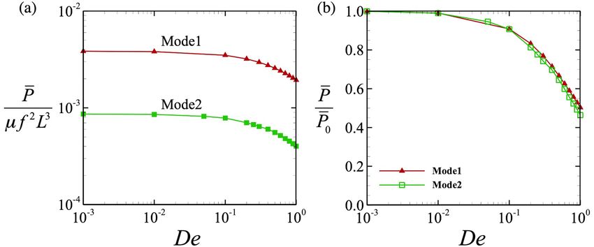
Micromachines 2019, 10, 78                                                                               2 of 9

that stiffer networks enhance the velocity of the swimmer. Although a number of researchers have
investigated sperm cells swimming through a viscoelastic liquid, many questions remain unanswered.
In particular, the efficiency and locomotive power of sperm in a viscoelastic fluid have not been
studied. As viscoelastic fluid can easily be found in the human body, knowledge about the efficiency
of locomotion through such media should be improved to further our understanding of reproduction
and our ability to fabricate micro-robots capable of operating in biological environments.
     In this study, we carried out a numerical investigation of sperm cells swimming through
viscoelastic fluid. The viscoelastic fluid was modeled by a linear Maxwell fluid. We evaluated
the swimming speed and efficiency whilst varying the Deborah number. In Section 2, we explain the
equations governing the motion and our numerical algorithm. Our results are presented in Section 3.
Finally, we conclude the paper in Section 4.

2. Governing Equations and Numerical Methods
    In this section, we explain the equations governing the motion of the sperm as well as our
numerical methods. Details of the fluid mechanics of a Maxwell fluid in the low-Reynolds number
regime can be found in [14,15], and we explain it briefly here.

2.1. Green’s Function for a Linear Maxwell Fluid
     We assumed that a sperm cell was immersed in an unbounded linear Maxwell fluid. We estimated
the Reynolds number of the sperm swimming through the fluid to be much smaller than unity [1].
Hence, we assumed that the fluid motion was a Stokes flow. The deviatoric stress tensor of the Maxwell
fluid is defined as:
                                               ∂
                                         1+λ        τ = 2µD,                                       (1)
                                               ∂t
where τ is the deviatoric stress of the fluid, λ is the relaxation time, and µ is the viscosity. D is the rate
of deformation tensor, which is defined as:
                                                                  !
                                                  1 ∂vi      ∂v j
                                           Dij =          +         ,                                      (2)
                                                  2 ∂x j     ∂xi

where v is the velocity of the fluid. By introducing the invertible linear operator L = µ(1 + λ∂/∂t)−1 ,
the momentum equation of the Maxwell fluid with a point force F can be written as [15]:

                                       ∂p      ∂2 v i
                                   −       +L         + δ(x, t; xs , ts ) Fi = 0,                          (3)
                                       ∂xi    ∂xk ∂xk

where p is the pressure and δ(x,t) is the delta distribution function in space and time, so that the point
force F is concentrated at a certain point xs and time ts . By using Green’s functions, the singularity
solution of Equation (3) is given by [15]:

                                 ∂P j         ∂2 Jij
                             −        Fj + L         F + 8πδ(x, t; xs , ts )δij Fj = 0,                    (4)
                                 ∂xi         ∂xk ∂xk j

where P (x,t; xs ,ts ) and J(x,t; xs ,ts ) are the pressure kernel and the Stokeslet for the Maxwell fluid,
respectively, which are singular at xs and ts :

                                       P j (x, t; xs , ts ) = P j0 (x; xs )δ(t − ts )                      (5)

and
                                    Jij (x, t; xs , ts ) = L−1 Jij0 (x; xs )δ(t − ts ),                    (6)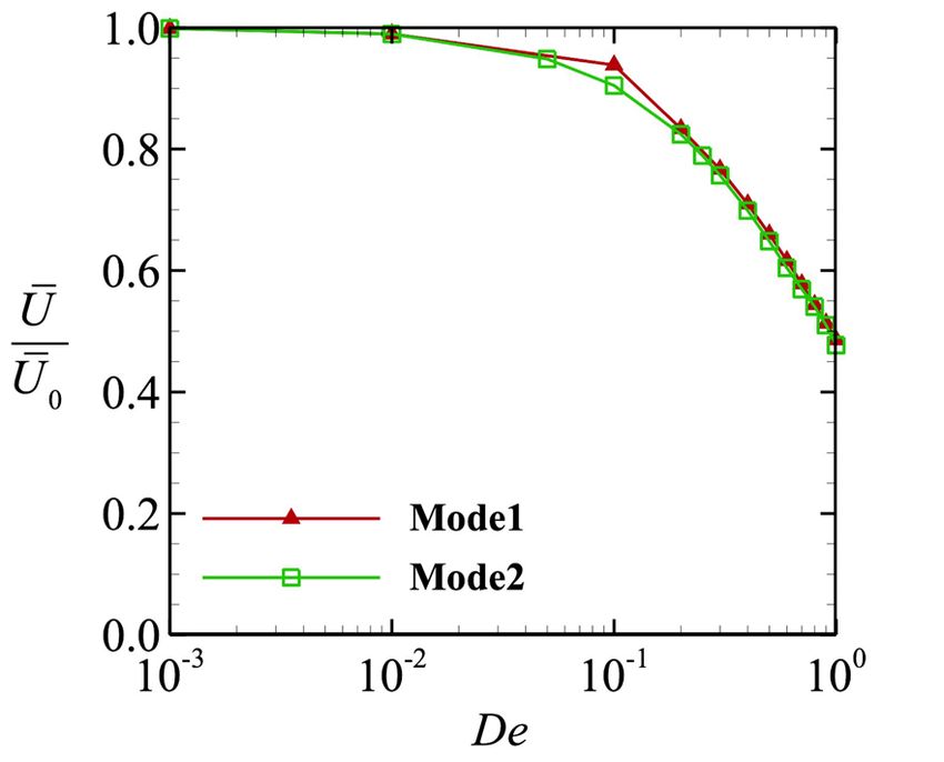
Micromachines 2019, 10, 78                                                                                                             3 of 9

where P 0 (x; xs ) and J0 (x; xs ) are the Green’s functions of a Newtonian fluid:
                                                                                  rj
                                                          P j0 (x; xs ) = 2                                                              (7)
                                                                                  r3
and
                                                                           δij  ri r j
                                                       Jij0 (x; xs ) =       3
                                                                               + 3 ,                                                     (8)
                                                                           r     r
where r = |r| and r = x – xs .

2.2. Boundary Integral Equation
     To describe the fluid dynamics of a sperm cell in viscoelastic fluid, we now introduce the boundary
integral equation. We were required to define an initial condition due to the presence of the time
derivative in Equation (4). We assumed, as a starting condition, that the dynamics were trivial for t
< 0 and that we had Stokes dynamics for t = 0 [15]. For t = ts (> 0), the flow field was calculated by
integrating the singularity solution with respect to time and space:

                                                              Zts Z
                                                       1
                                      vi (x, ts ) = −                     L−1 Jij0 δ(t − ts )q j dSdt,                                   (9)
                                                      8π              S
                                                              0

where q is the traction force per unit area, and S represents the surface of the cell.
      In this study, the slender-body theory [16] was applied to the motion of the flagellum. The
flagellum was modeled as a thin, curved rod with a length–radius ratio a/L = 3.57 × 10⁻³ [1], where
a is the flagellar radius and L is the length. Then, the flow field can be described by the following
boundary integral—the slender-body coupling formulation:

                                  Zts Z
                              1
                                                                                    Z
             vi (x, ts ) = −                      L−1 Jij0 δ(t − ts )q j dS +                         L−1 Kij0 δ(t − ts ) f j dl dt,   (10)
                             8π            head                                         f lagellum
                                  0

where f is the force per unit length of the flagellum, and K0 is the slender-body kernel [16]. The delta
distribution gives the limiting value of the time integral, and the boundary integral of the Maxwell
fluid is reduced to the Newtonian kernel with the leading time derivative:
                                                           Z
                                                   1 −1
                                                                                          Z
                             vi (x, ts ) = −         L                    Jij0 q j dS +                    Kij0 f j dl .               (11)
                                                  8π              head                        f lagellum

2.3. Flagellar Waveform and Head Geometry
     To accurately describe the flagellar waveform, we introduce an orthonormal body frame, ξ i , with
the origin at the head–tail junction. We assumed a rigid connection between the head and the flagellum,
and the minus ξ 1 -axis was set to coincide with the orientation vector. The waveform was specified a
priori for a given transformation in terms of the following sinusoidal function [17]:

                                        ξ 2 = A(ξ 1 ) cos 2π (ξ 1 /Lη (ξ 1 ) − t/T ),
                                                                                                                                       (12)
                                        ξ 3 = αA(ξ 1 ) sin 2π (ξ 1 /Lη (ξ 1 ) − t/T ),

where T is the period of the flagellar waveform, η is the wavelength (which can vary with respect to
ξ 1 ), and α is the chirality parameter. These parameters were selected such that they coincided with
experimental observations.
        An experimental study of the waveform of the human sperm flagellum was reported in [18,19].
In low-viscosity liquid, high apparent curvatures appeared along with whole flagellum, and the head
made repeated yawing motions. In high-viscosity liquid, on the other hand, a steeping wave appeared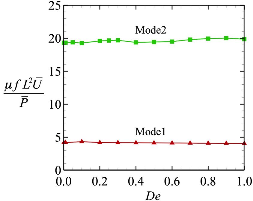
Micromachines 2019, 10, 78 4 of 9
near the tip of the flagellum and the yawing motion of the head was less pronounced. We defined two
different beating
Micromachines patterns
2019, 10, to express
x FOR PEER REVIEWthese different wave modes, as shown in Figure 1, by varying4 the of 9
− 1
wavelength η [17]: η = 1 for Mode 1, and η = 0.9613 − 0.038 tan (5ξ 1 − 4) for Mode 2. The amplitudes
The amplitudes
of the two wavesofwere
the two wavestowere
adjusted matchadjusted to match speed
the swimming the swimming speed influid.
in a Newtonian a Newtonian fluid.
If the chirality
If the chirality
parameter, α, isparameter, α,=is0.25
also set to α also[18],
set then
to α the
= 0.25 [18],makes
sperm then the sperm
rolling makesasrolling
motions motions as it
it swims.
swims.
Figure 1. Flagellar beat with (a) Mode 1 and (b) Mode 2. Top panels are seen from the top, whereas
bottom panels
panels are
are seen
seenfrom
fromthetheside.
side.Temporal
Temporalflagellar profiles
flagellar areare
profiles shown by by
shown different colors:
different redred
colors: for
t/T = 0.0, green for t/T = 0.2, blue for t/T = 0.4, magenta for t/T = 0.6, and black for t/T = 0.8,
for t/T = 0.0, green for t/T = 0.2, blue for t/T = 0.4, magenta for t/T = 0.6, and black for t/T 0.8, where T
is the beat period.
Both human
Both human and
and bull
bull sperm
sperm are
are similar
similar to
to asymmetric
asymmetric ellipsoids
ellipsoids [1].
[1]. We
We mimicked
mimicked the
the elliptical
elliptical
sperm head
sperm head using
using the
the following
following mapping
mapping function
function [10]:
[10]:
sp sp ,
sp cc2 XX2 sp X X3
X1 =X X
1
, X=2sp =c + c 2− 2X /`, , XX3sp3 = = c 3+ X, /` ,
1= X X
1 2
(13)
(13)
1c + c2 − X 1 c3 +3X 1 1
1 2 1
sp is a point on the head of the sperm, X is a point on the sphere with radius `, and c , c , and
where X
where Xsp is a point on the head of the sperm, X is a point on the sphere with radius , and c11, c22, and
c3 are non-dimensional shape parameters. The parameters were set to `/L = 4.17 × 10⁻²−2, c1 = 3.0, c2 =
c3 are non-dimensional shape parameters. The parameters were set to L = 4.17 × 10 , c1 = 3.0, c2 =
2.0, and c3 = 4.0 to ensure that the morphology accurately reflected a human sperm cell.
2.0, and c3 = 4.0 to ensure that the morphology accurately reflected a human sperm cell.
2.4. Numerical Procedure
2.4. Numerical Procedure
To express the locomotion of the sperm cell, we assumed that the cell moves rigidly. One motion
To express isthe
of the flagellum locomotion
defined of the(12).
by Equation sperm
Thecell, we assumed
velocity at a pointthatxs onthe
thecell
cell moves rigidly. One
can be decomposed
motion
as: of the flagellum is defined by Equation (12). The velocity at a point xs on the cell can be
decomposed as: v(xs ) = V + Ω ∧ r̂ + v f la (xs , t), (14)
where V is the translational velocity, Ω is the angular velocity, r̂ =
, xs − xg , and xg is the center-of-mass
(14)
fla
of the head. The velocity of the flagellum wave is v (xs ,t), a function of the point of interest and time.
where x Vis is
When s
the translational
located velocity,
on the cell head, then vflaΩis is thetoangular
equal velocity,
zero. When r̂ = xs on
x is located
s
− xthe
g
, flagellum,
and xg is then
the
vfla is determined
center-of-mass by the
of the time
head. Thederivative
velocity of
of Equation (12). wave is vfla (xs,t), a function of the point of
the flagellum
We and
interest solved theWhen
time. resistance
xs is problem
located ondefined in head,
the cell Equations
then (11)
vfla isand (14)to
equal with respect
zero. Whentoxthe unknowns
s is located on
theΩflagellum,
V, and the tractions
then v is
fla q and f . The head
determined andtime
by the flagellum wereofdiscretized
derivative into 1280 triangular meshes
Equation (12).
and 200We curved
solved segments by spline
the resistance interpolation.
problem defined in TheEquations
surface integral of Equation
(11) and (14) with(11) was solved
respect to the
using Gaussian
unknowns V, Ωnumerical
and the integration,
tractions q while
and f.the finite
The time
head difference
and flagellumscheme
werewas applied tointo
discretized the 1280
time
triangular meshes and 200 curved segments by spline interpolation. The surface integral of Equation
(11) was solved using Gaussian numerical integration, while the finite time difference scheme was
applied to the time derivative. We assumed the following force-free and torque-free conditions so
that we could express the free-swimming sperm cell as:
q dS + f dl = 0, q ∧ r̂ dS + f ∧ r̂ dl = 0 . (15)Micromachines 2019, 10, 78 5 of 9
derivative. We assumed the following force-free and torque-free conditions so that we could express
the free-swimming sperm cell as:
Z Z Z Z
qdS + fdl = 0, q ∧ r̂dS + f ∧ r̂dl = 0. (15)
The above equations were also discretized so that Gaussian numerical integration could be performed.
Once V and Ω were determined, the point of interest was updated using the second-order Runge–Kutta
method. For more detail about the numerical method, please refer to our previous study [10].
We then introduced an important parameter, the Deborah number, which represents the elasticity
and viscosity ratio of the viscoelastic fluid, and is characterized by the relaxation time λ. In this
study, the Deborah number is defined as De = ωλ, where ω is the angular frequency of the flagellar
beat. In the small-Deborah number regime, DeMicromachines 2019,
Micromachines 2019, 10,
10, 78
x FOR PEER REVIEW 66 of
of 99
0.010
(a) (c)
0.005 Mode1
y
0.000
L
-0.005 Mode2
Wave Mode1 -0.010
-0.1 0.0 0.1 0.2 0.3 0.4
x/L
(b)
(d)
Mode1 Mode2
U fL 0.01612 0.01672
V fL 0.01606 0.01664
Wave Mode2
Figure
Figure 2. Swimmingofofthe
2. Swimming the sperm
sperm model
model in ainNewtonian
a Newtonian fluid.
fluid. (a) Superimposed
(a) Superimposed imageimage of the
of the model
model during one period with Mode 1. (b) Superimposed image with Mode
during one period with Mode 1. (b) Superimposed image with Mode 2. (c) Trajectories of 2. (c) Trajectories of the
the
center-of-mass of the head in the (x,y)-plane during 20 beats. The dotted arrow indicates
center-of-mass of the head in the (x,y)-plane during 20 beats. The dotted arrow indicates the averagethe average
in-plane
in-plane displacement.
displacement.(d)(d)Time-averaged
Time-averaged swimming
swimmingspeeds withwith
speeds two different definitions.
two different The values
definitions. The
are averaged across 20 beats and normalized by the beat frequency f (= 1/T, where T is
values are averaged across 20 beats and normalized by the beat frequency f (= 1/T, where T is thethe beat period)
beat
and the flagellar
period) length L.length L.
and the flagellar
The swimming speeds U and V of the two beat modes are shown in Figure 2d. As the trajectories
3.2. Swimming Motion of a Sperm Cell in a Maxwell Fluid
were almost straight, the values of U and V were similar between both beat modes, as shown in
Figure Next,
2d. we considered a sperm cell swimming through a linear Maxwell liquid. Since the impact
of the initial conditions decays over the timescale of the relaxation time λ, we limit our discussion to
3.2. Swimming
the physical Motion
values of a Sperm
observed Cellthe
after in first
a Maxwell
periodFluid
T, t ≥ T, which was sufficiently large for the initial
conditions to decay.
Next, we considered a sperm cell swimming through a linear Maxwell liquid. Since the impact
of theThe temporal
initial flowdecays
conditions fields and
overpressure distributions
the timescale at time t time
of the relaxation = T with
λ, weDelimit
= 0.0our
anddiscussion
De = 1.0 are to
shown in Figure 3. Note that the pressure field was determined by the kernel shown
the physical values observed after the first period T, t ≥ T, which was sufficiently large for the initial in Equation (5).
As shown in
conditions to Figure
decay. 3, high pressure was observed in the forepart of the flagellum/head movement,
whileThethetemporal
negative flowpressure appeared
fields at the distributions
and pressure rear in all cases. In the
at time t =case of wave
T with De =mode
0.0 and1 with
De =De1.0=are
0.0
(Figure 3a), the pressure was enhanced within the region of r/L < 0.1 along
shown in Figure 3. Note that the pressure field was determined by the kernel shown in Equation (5). with the whole flagellum,
thatshown
As is, theinred region3,in
Figure Figure
high 3, where
pressure wasr observed
is the distance
in thefrom the nearest
forepart flagellum/head surface
of the flagellum/head movement, and
L is the flagellar length. By increasing the Deborah number, the high-pressure
while the negative pressure appeared at the rear in all cases. In the case of wave mode 1 with De = 0.0 region shrank to near
the surface
(Figure (r/Lpressure
3a), the < 0.05, seewasFigure
enhanced3b). within
Accordingly,
the regionthe of
flow
r/Lgenerated
< 0.1 alongby thethe
with sperm’s
wholeswimming
flagellum,
diminished as the Deborah number increased. The same tendency was observed
that is, the red region in Figure 3, where r is the distance from the nearest flagellum/head surface in wave Modeand2
(Figure 3c,d), although both flow and pressure fields were different between
L is the flagellar length. By increasing the Deborah number, the high-pressure region shrank to near the two modes. In this
study, the flagellum waveform was prescribed, that is, the beating
the surface (r/L < 0.05, see Figure 3b). Accordingly, the flow generated by the sperm’s swimmingspeed was defined, and the
traction wasas
diminished determined
the Deborah based on theincreased.
number time derivatives
The same according
tendency to Equation (11). The
was observed traction
in wave Modeforce 2
decreased with the flagellar velocity. As small traction forces cannot produce
(Figure 3c,d), although both flow and pressure fields were different between the two modes. In this strong fluid flow, the
flow was
study, the weak in the
flagellum high-De regime.
waveform was prescribed, that is, the beating speed was defined, and the traction
was determined based on the time derivatives according to Equation (11). The traction force decreased
with the flagellar velocity. As small traction forces cannot produce strong fluid flow, the flow was
weak in the high-De regime.Micromachines 2019, 10, 78 7 of 9
Micromachines 2019, 10, x FOR PEER REVIEW 7 of 9
Micromachines 2019, 10, x FOR PEER REVIEW 7 of 9
(a)(a) (b)
(b)
p pμ μf f
0.1
0.1
Wave Mode 1, De = 0.0 Wave Mode 1, De = 1.0
Wave Mode 1, De = 0.0 Wave Mode 1, De = 1.0
(c)(c) (d)
(d)
- 0.1
- 0.1
Wave Mode 2, De = 0.0 Wave Mode 2, De = 1.0
Wave Mode 2, De = 0.0 Wave Mode 2, De = 1.0
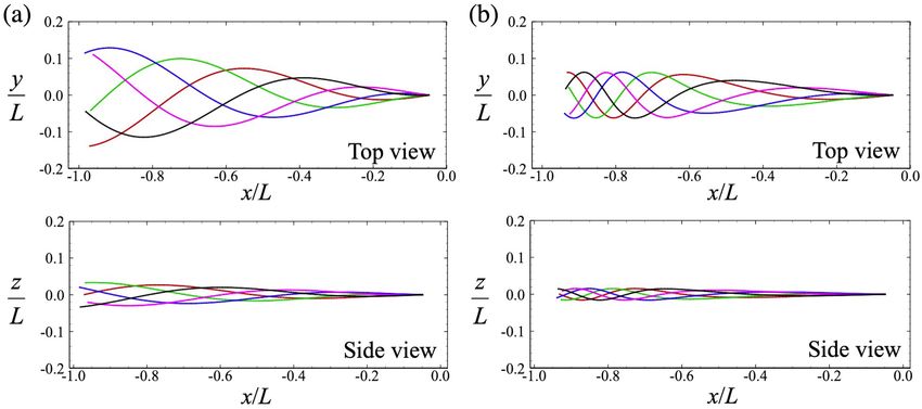
Figure3. 3. Temporal flow and pressure fields
at at t T= with
T with
DeDe = 0.0 and 1.0; (a,b) show wave Mode 1
Figure
Figure 3. Temporal
Temporal flow
flow and
and pressure
pressure fields
fields at tt =
=T with De == 0.0
0.0 and
and 1.0;
1.0; (a,b)
(a,b) show
show wave
wave Mode
Mode 11
and
and (c,d)
(c,d) show
show wave
wave Mode
Mode 2. 2. The
The contours
contours represent
represent pressure,
pressure, which
which is is normalized
normalized by by viscosity
the the viscosity
µ
and (c,d) show wave Mode 2. The contours represent pressure, which is normalized by the viscosity
μ and
and frequency
frequency f. f.
μ and frequency f.
TheTheaverage
averageswimming
swimming speeds
speeds U with
U with different values
different of De of
values areDe
shown in Figure
are shown 4. The4.
in Figure value
The was
value
The average swimming speeds U with different values of De are shown in Figure 4. The value
averaged in the range
was averaged in the10T ≤ t ≤10T
range 20T≤and
t ≤ normalized by the swimming
20T and normalized by the speed through
swimming a Newtonian
speed through a
was averaged in the range 10T ≤ t ≤ 20T and normalized by the swimming speed through a
fluid U 0 . In fluid
Newtonian U . In the small-Deborah
the small-Deborah number region DeMicromachines 2019, 10, 78 8 of 9
3.3. Power and Swimming Efficiency
To see the effect of the Deborah number in more detail, we investigated the power generated by
the locomotion. The power P due to the cellular locomotion is:
Z Z
P= v · qdS + v · fdl. (18)
Micromachines 2019, 10, x FOR PEER REVIEW 8 of 9
The time-averaged powers for the different wave modes are shown in Figure 5a. For all values of
P = v ⋅ q dS + v ⋅ f dl . (18)
De tested, the power P of Mode 1 was always higher than that of Mode 2. However, the two curves
matched when Thewe normalizedpowers
time-averaged the value bydifferent
for the the power modesDe
wavewhen are→ 0 (i.e.,
shown at P0 ),5a.asFor
in Figure shown in Figure 5b.
all values
of De tested, the
We then investigated power
the P of Mode
efficiency 1 was
of the always higher
locomotion. The than that of Mode
efficiency was 2.defined
However, bythe
thetwoswimming
we normalized the value by the power when De → 0 (i.e., at P00), as shown in
speed percurves
unit matched
power, µfL when
2 U/P, where µ is the viscosity, f is the beat frequency, and L is the flagellar
Figure 5b. We then investigated the efficiency of the locomotion. The efficiency was defined by the
length. The results are shown in Figure 6, where we can clearly see that the efficiency was almost
swimming speed per unit power, μfL22U/P, where μ is the viscosity, f is the beat frequency, and L is
independent of De, length.
the flagellar and the
Thevalue
resultsbecame
are shown constant.
in Figure When
6, wherethe we efficiency was
can clearly see thatfixed, the tendency of
the efficiency
the swimming speed
was almost to decay of
independent De, De
with andwas less dependent
the value became constant. on the Whenwave pattern. was
the efficiency Thus, thethe
fixed, swimming
tendency of the swimming speed to
speed varied in the same way in both wave modes. decay with De was less dependent on the wave pattern. Thus,
the swimming speed varied in the same way in both wave modes.
Power
Figure 5.Figure due todue
5. Power thetolocomotion:
the locomotion:(a) (a)The
The value was
value was normalized
normalized byviscosity
by the the viscosity µ, the beat
μ, the beat
frequency f, and the flagellar length L. (b) Power was normalized by P in a Newtonian
frequency f, and the flagellar length L. (b) Power was normalized by P0 in a Newtonian fluid.
0
0 fluid.
Figure
Figure 6. Swimmingefficiency
6. Swimming efficiency asas
a function of De.
a function of De.
4. Conclusions
4. Conclusion
In this study, we numerically investigated a sperm cell swimming in a linear Maxwell fluid in
In this study, we numerically investigated a sperm cell swimming in a linear Maxwell fluid in the
the small-De regime (De < 1.0). We found that, for the given waveform, the efficiency of the motion
small-De regime (De < 1.0). We found that, for the given waveform, the efficiency of the motion remained
remained constant as the Deborah number varied. The fixed efficiency diminished the effect of the
constant as the pattern
wave Deborah on number varied.
the decrease The fixedspeed
in swimming efficiency diminished
with De. the effect
These findings couldof
bethe wavetopattern on
relevant
the decrease in swimming
one-way speed
fluid–structure with De.
interaction andThese
may befindings
helpful tocould be relevant
researchers designingtomicro-swimmers
one-way fluid–structure
in
viscoelastic fluids with prescribed velocity conditions. For further study, to
interaction and may be helpful to researchers designing micro-swimmers in viscoelastic fluids with understand the
physiology of sperm swimming, we must consider full fluid–structure interactions by developing a
prescribed velocity conditions. For further study, to understand the physiology of sperm swimming, we
mechanical model of the inner structure of the flagellum.
must consider full fluid–structure interactions by developing a mechanical model of the inner structure of
the flagellum.Micromachines 2019, 10, 78 9 of 9
Author Contributions: T.O. and T.I. designed the research; T.O. performed the simulation; T.O. and T.I. analyzed
the data; T.O. and T.I. wrote the paper.
Funding: The authors acknowledge the support of JSPS KAKENHI (Grants No. 18K18354 and 17H00853). We
also acknowledge Mr. Eisaku Shimomura, who took the data in early stages of this study.
Conflicts of Interest: The authors declare no conflict of interest. The founding sponsors had no role in the design
of the study; in the collection, analyses, or interpretation of data; in the writing of the manuscript, and in the
decision to publish the results.
References
1. Gaffney, E.A.; Gadêlha, H.; Smith, D.J.; Blake, J.R.; Kirkman-Brown, J.C. Mammalian sperm motility:
Observation and theory. Annu. Rev. Fluid Mech. 2011, 43, 501–528. [CrossRef]
2. Hyakutake, T.; Suzuki, H.; Yamamoto, S. Effect of non-Newtonian fluid properties on bovine sperm motility.
J. Biomech. 2015, 48, 2941–2947. [CrossRef] [PubMed]
3. Khalil, I.S.M.; Dijkslag, H.C.; Abelmann, L.; Misra, S. MagnetoSperm: A microrobot that navigates using
weak magnetic fields. Appl. Phys. Lett. 2014, 104, 223701. [CrossRef]
4. Kaynak, M.; Ozcelik, A.; Nourhani, A.; Lammert, P.E.; Crespi, V.H.; Huang, T.J. Acoustic actuation of
bioinspired microswimmers. Lab Chip 2017, 17, 395–400. [CrossRef] [PubMed]
5. Smith, D.J.; Gaffney, E.A.; Blake, J.R.; Kirkman-Brown, J.C. Human sperm accumulation near surfaces:
A simulation study. J. Fluid Mech. 2009, 621, 289–320. [CrossRef]
6. Ishimoto, K.; Gaffney, E.A. A study of spermatozoan swimming stability near a surface. J. Theor. Biol. 2014,
360, 187–199. [CrossRef] [PubMed]
7. Gadêlha, H.; Gaffney, E.A.; Smith, D.J.; Kirkman-Brown, J.C. Nonlinear instability in flagellar dynamics: A
novel modulation mechanics in sperm migration? J. R. Soc. Interface 2010, 7, 1689–1697. [CrossRef] [PubMed]
8. Kantsler, V.; Dunkel, J.; Blayney, M.; Goldstein, R.E. Rheotaxis facilitates upstream navigation of mammalian
sperm cells. eLife 2014, 3, e02403. [CrossRef] [PubMed]
9. Ishimoto, K.; Gaffney, E.A. Fluid flow and sperm guidance: A simulation study of hydrodynamic sperm
rheotaxis. J. R. Soc. Interface 2015, 12, 20150172. [CrossRef] [PubMed]
10. Omori, T.; Ishikawa, T. Upward swimming of a sperm cell in shear flow. Phys. Rev. E 2016, 93, 032402.
[CrossRef] [PubMed]
11. Elgeti, J.; Winkler, R.G.; Gompper, G. Physics of microswimmers—Single particle motion and collective
behavior. Rep. Prog. Phys. 2015, 78, 056601. [CrossRef] [PubMed]
12. Ishimoto, K.; Gadêlha, H.; Gaffney, E.A.; Smith, D.J.; Kirkman-Brown, J.C. Human sperm swimming in a
high viscosity mucus analogue. J. Theor. Biol. 2018, 446, 1–10. [CrossRef] [PubMed]
13. Wróbel, J.K.; Lynch, S.; Barrett, A.; Fauci, L.; Cortez, R. Enhanced flagellar swimming through a compliant
viscoelastic network in Stokes flow. J. Fluid Mech. 2016, 792, 775–797. [CrossRef]
14. Ishimoto, K.; Gaffney, E.A. Boundary element methods for particles and microswimmers in a linear
viscoelastic fluid. J. Fluid Mech. 2017, 831, 228–251. [CrossRef]
15. Smith, D.J.; Gaffney, E.A.; Blake, J.R. Mathematical modelling of cilia-driven transport of biological fluids.
Proc. R. Soc. A 2009, 465, 2417–2439. [CrossRef]
16. Tornberg, A.-K.; Shelly, M.J. Simulating the dynamics and interactions of flexible fibers in Stokes flows.
J. Comput. Phys. 2004, 196, 8–40. [CrossRef]
17. Dresdner, R.D.; Katz, D.F. Relationships of mammalian sperm motility and morphology to hydrodynamic
aspects of cell function. Biol. Reprod. 1981, 25, 920–930. [CrossRef] [PubMed]
18. Ishijima, S.; Hamaguchi, M.S.; Naruse, M.; Ishijima, A.; Hamaguchi, Y. Rotational movement of a
spermatozoon around its long axis. J. Exp. Biol. 1992, 163, 15–31. [PubMed]
19. Friedrich, B.M.; Riedel-Kruse, I.H.; Howard, J.; Julicher, F. High-precision tracking of sperm swimming
fine structure provides strong test of resistive force theory. J. Exp. Biol. 2010, 213, 1226–1234. [CrossRef]
[PubMed]
© 2019 by the authors. Licensee MDPI, Basel, Switzerland. This article is an open access
article distributed under the terms and conditions of the Creative Commons Attribution
(CC BY) license (http://creativecommons.org/licenses/by/4.0/).You can also read