Time scales and rheology of visco-cohesive granular flows
←
→
Page content transcription
If your browser does not render page correctly, please read the page content below
EPJ Web of Conferences 249, 03044 (2021)                                                                https://doi.org/10.1051/epjconf/202124903044
Powders and Grains 2021

      Time scales and rheology of visco-cohesive granular flows

      Farhang Radjai1,⇤
      1
          CNRS, LMGC, University of Montpellier, 163 rue Auguste Broussonnet, F-34095 Montpellier, France

                     Abstract. In the presence of viscous and cohesive interactions between particles, a granular flow is governed
                     by several characteristic time and stress scales that determine its rheological properties (shear stress, packing
                     fraction, e↵ective viscosities). In this paper, we revisit and extend the scaling arguments used previously for
                     dry cohesionless granular flows and suspensions. We show that the rheology can be in principle described by a
                     single dimensionless control parameter that includes all characteristic times. We also briefly present simulation
                     results for 2D sheared suspensions and 3D wet granular flows where the e↵ective friction coefficient and packing
                     fraction are consistently described as functions of this unique control parameter.

      1 Introduction                                                            or stresses come into play, a closer examination of such
                                                                                mechanisms becomes necessary. For example, for dense
      Scaling arguments have been successfully used for a long                  suspensions of particles in a liquid, both particle inertia
      time in the field of granular materials. For example, as                  and liquid viscosity need to be considered in addition to
      perfect rigid particles and friction law involve no intrinsic             the confining stress. Numerical simulations suggest that
      stress scale, the shear stresses in quasi-static flows are con-           the rheology can still be described by a single dimension-
      tained in a Coulomb cone, which bears on the description                  less control parameter involving the ratio of a linear com-
      of the shear strength in terms of stress ratios [1]. Hence,               bination of viscous and kinetic stresses to the confining
      the ratio of shear stress to the normal stress is an e↵ective             stress [4, 5]. On the other hand, in the case of visco-
      friction coefficient µ whose evolution with shear strain de-              cohesive granular materials, the cohesive stress is added
      scribes the quasi-static rheology together with that of di-               to the confining stress and a single control parameter is
      latancy, which due to rate independence in the quasi-static               defined from four di↵erent stress scales [6]. Besides un-
      limit, is also a ratio of volumetric strain to shear strain.              derstandable arguments such as delineating the shear-rate
      We refer to such states as quasi-static flow states (QSFS).               dependent internal stresses from shear-rate independent
      The scaling argument was also used to rationalize the be-                 stresses, the rationale behind such an “additive rheology"
      havior of inertial flows by considering that a dry cohe-                  needs to be clarified from a particle-scale standpoint [7].
      sionless flow driven by a shear rate ˙ involves two time
      scales, and only their ratio is relevant for the evolution of
      µ and [2]: 1) shear time ti = ˙ 1 and 2) relaxation time
      t p = d(⇢ s / p )1/2 of a particle of mass density ⇢ s and di-
      ameter d under the action of a confining stress p . The                        In the following, I first discuss a physical pic-
      ratio is the inertial number I = t p /ti = ˙ d(⇢ s / p )1/2 , and         ture of steady granular flows as a continuous pertura-
      the rheology is described by the functions µ(I) and (I).                  tion/relaxation process with a reference state (or ground
      In a similar vein, in a suspension of particles immersed in               state) defined by the confining stress. In this framework,
      a viscous fluid, if the viscous drag stress ⌘ f ˙ , where ⌘ f is          I show why mean contact forces can be used to express
      the fluid dynamic viscosity, is considered together with a                the particle relaxation times. Then, I introduce the con-
      confining stress p exerted on the granular phase, the rhe-                cept of cohesive stress arising from active adhesion forces
      ology is described by the functions µ(J) and (J) of the                   at the contact points between particles, and argue that the
      dimensionless number J = ⌘ f ˙ / p [3].                                   cohesive stress in dense granular flows plays the same role
           In the above examples the use of dimensionless num-                  as the confining stress, defining together a time scale that
      bers stems from a general dimensional analysis (unit in-                  characterizes the reference flow state. Next, I discuss par-
      dependence) or objectivity principle (frame independence                  ticle transition times for kinetic and viscous stresses and
      requiring µ to be defined from stress invariants) without                 the meaning of a combined visco-inertial transition time.
      referring to the underlying physical mechanisms, which                    Finally, I show how a single dimensionless number Im is
      are complex and often characterized by broad statistical                  naturally defined as a number characterizing the ratio of
      distributions of the particle momenta, contact forces, col-               the transition rate to the relaxation rate, and briefly present
      lision times. . . ). However, when more characteristic times              simulation results in which µ and collapse on a master
           ⇤ e-mail: franck.radjai@umontpellier.fr                              curve when plotted as a function of Im .
           A video is available at https://doi.org/10.48448/2vfd-4d39
© The Authors, published by EDP Sciences. This is an open access article distributed under the terms of the Creative Commons Attribution License 4.0
(http://creativecommons.org/licenses/by/4.0/).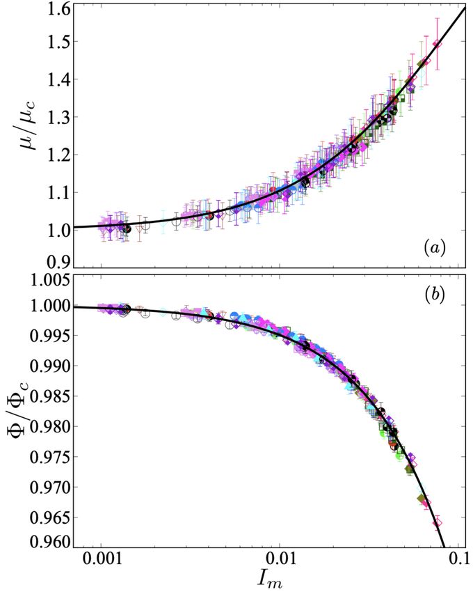
EPJ Web of Conferences 249, 03044 (2021)                                                                   https://doi.org/10.1051/epjconf/202124903044
Powders and Grains 2021

                                                                               accommodated. The transition between two stable config-
                                                                               urations is governed by the shear rate whereas relaxation
                                                                               to a new configuration is controlled by the confining stress.
                                                                                    For the estimation of the relaxation time, we need an
                                                                               evaluation of the force fluctuations. The total force F(i)   ~
                                                                               on particle i changes as a result of the evolution of contact
                                                                               forces f~i j exerted by contact neighbors j. As we seek the
                                                                               connection with the imposed stress p , let us consider the
                                                                                                                                    P
                                                                               yy-component of the tensor moment Myy (i) = j fy,i j ry,i j
                                                                               of particle i, where ry,i j is the y-component of the posi-
                                                                               tion vector of the contact (i j). The tensor moment inside
                                                                               a volume V is simply the sum of the tensor moments of
      Figure 1. (a) Simple shear geometry; (b) Local particle environ-         the particles belonging to V and it can be shown that its
      ment.                                                                    density tends to the Cauchy tensor as the number of par-
                                                                                                     P
                                                                               ticles increases V1 i Myy (i) ! yy [9]. Near equilibrium,
                                                                               where the forces are nearly balanced, the tensor moment
      2 Perturbation/relaxation process                                        M(i) of each particle is independent of the choice of the
                                                                               origin for the contact position vectors ~ri j . If the origins of
      Let us focus on the simple shear geometry of Fig. 1(a).                  the contact vectors for each particle are taken at their cen-
      The granular flow is subjected to periodic boundary con-                 ters, the particle tensor moments are Myy (i) = Z(i)h fy cy ii
      ditions along the flow (x direction) and driven by a shear               where ~ci j = ~ri ~ri j is the contact vector (drawn from parti-
      strain rate ˙ . The vertical stress p is the confining pres-             cle center to the contact point), the average h· · · ii denotes
      sure, the only stress applied externally on the particles                summation over all contacts of particle i, and Z(i) is the
      (not on the liquid) and perpendicular to the flow (y di-                 number of its contacts. The Cauchy stress tensor (here yy-
      rection). The memory of the initial packing state is lost                element) can therefore be expressed as
      upon shearing, and the steady flow state implies the bal-
      ance of external and internal stresses. Hence, yy = p ,                         yy   = n p hMyy (i)i = n p hZ(i)h fy cy ii i = 2nc h fy cy i    (1)
      and yx = xy = ⌧ is the shear stress. The ratio µ = ⌧/ p                  where n p = N p /V is the number density of particles and
      characterizes the steady stress state. Both µ and depend                 nc = Nc /V = Zn p /2 is the number density of contacts.
      on the material properties (friction coefficient between par-            This expression means that the stress tensor is an ensemble
      ticles, particle shapes and size distributions) and the con-             average (NPT ensemble) over single particle tensor mo-
      trol parameters p and ˙ . The particles are assumed to be                ments weighted by their numbers of contacts Z(i) (local
      perfectly rigid so that the only material parameters at the              coordination numbers). It can be described statistically by
      particle scale are the mean particle diameter d and the par-             considering one particle and the probability distributions
      ticle density ⇢ s or mean particle mass ⇢ s d3 . Here, we are            of forces, coordination numbers and contact directions.
      only interested in the role of control parameters in combi-                    Let us now consider the fluctuations fy of the verti-
      nation with fixed material parameters.                                   cal force component. To simplify the derivation, we as-
           A strict QSFS means that the particles follow ex-                   sume spherical particles of average radius R although it
      actly the displacements imposed by the uniform shear rate                can easily be extended to more general particle shapes. We
      (affine displacement). In other words, for a particle i at               thus have cy = R sin ✓. Note that fy = ( fn cos ✓ + ft sin ✓)
      a position ~r(i), the velocity components are v x (i) = ˙ ry (i)                                        P
                                                                               is a signed variable and j fy,i j ' 0 due to equilibrium.
      and vy (i) = 0. Such a motion is obviously forbidden due                 Hence h fy i = 0 and fy = h fy2 i1/2 . The tensor moment
      to steric exclusions between particles. Hence, nonaffine                 can be evaluated from the components under the general
      displacements ~s(i) are developed to accommodate particle                assumption that the forces and contact orientations are
      motions [8]. The motion can be described as the sum of                   not correlated with the contact directions ✓, implying an
      affine and nonaffine components: v x (i) = ˙ ry (i) + ṡ x (i) and       isotropic contact network. It can be shown that the con-
      vy (i) = ṡy (i), with h ṡ x (i)i = h ṡy (i)i = 0. The nonaffine       tact network anisotropy is of second order. Therefore
      displacement field is observed to be highly correlated in                h fy cy i = Rh fn sin2 ✓ + ft sin ✓ cos ✓i = R2 h fn i. We may al-
      space, but disappears after a short time before a new pat-               ternatively evaluate it from the Pearson correlation K f c =
      tern appears. This process clearly shows that the overall                                                                              p
                                                                               h fy cy i/( fy cy ). We have cy = hR2 cos2 ✓i1/2 = R/ 2.
      shear deformation is composed of periods of the buildup of
                                                                               Hence,
      correlated motions and short periods of relaxation. At the
      scale of a single particle, the nonaffine displacements in-                                      1                    1        p
                                                                                             fy = p            h fn i = p                 = kd2   p   (2)
      duced by the motions of all particles implies the variation                                     2K f c                2K f c nc R
      of the contact forces acting on the particles by its neigh-
      bors. During its motion, the particle probes the force net-              with                                   p
      work, which is highly inhomogeneous. The force acting                                                            2⇡
                                                                                                               k=            .                        (3)
      on the particle are balanced during the buildup of collec-                                                    3Z K f c
      tive motions, but becomes unstable whenever the changes                  This prefactor is of the order 0.4 and its variations are
      in nonaffine components of the displacements are no more                 small. Equation (2) shows that the force fluctuations are

                                                                           2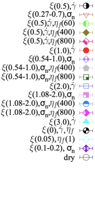
EPJ Web of Conferences 249, 03044 (2021) https://doi.org/10.1051/epjconf/202124903044
Powders and Grains 2021
proportional to the average normal force and confining
stress. This is consistent with the nearly exponential dis-
tribution of force components, which implies that standard
deviation is equal to the mean. Since fy is signed, its stan-
dard deviation is two times h| fy |i. These two viewpoints
correspond respectively either to set of particles inside a
granular packing or to a moving particle experiencing lo-
cal force variations.
For the evaluation of the relaxation time one can thus
use d2 p instead of fy . For an acceleration equal to a =
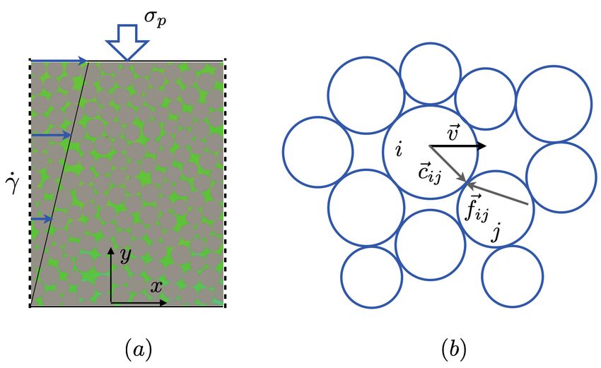
fy /m, the particle moves a distance at2 /2 during a time t. Figure 2. E↵ective friction coefficient in simulated wet materials
A coarse-grained relaxation time can be defined assuming in quasi-static flow as a function of cohesion number.
fluctuations of the order of fy and distances of the order
of particle diameter d. The relaxation time is the time for
a particle to move a distance equal to its own diameter [2]: 2
Replacing fy by cd in equation (4), we get the relax-
!1/2 ation time
md !1/2
tx = (4) ⇢s
fy tc = d (8)
c
Hence, for an external confining pressure p , the force
However, the cohesive relaxation time does not make
fluctuation is d2 p and relaxation time is given by t p =
✓ ◆1/2 ✓ ◆1/2 sense alone in the presence of a confining stress p . Both
m
p and c tend to counterbalance the e↵ect of shear-
⇢s
pd
= d p
, where we set m ' ⇢ s d3 .
The particles are driven by the shear rate ˙ , and the induced perturbations. By stress additivity, we therefore
transition time is the time required for a particle to move a consider n = p + c as the reference stress, and the
distance equal to its own diameter under the action of the normal relaxation time is given by
kinetic or inertial stress i = ⇢ s (d ˙ )2 . Replacing fy by !1/2
⇢s tp
d2 i in equation (4), we get the kinetic time ti tn = d = (9)
c+ p (1 + ⇠)1/2
!1/2
md
tx = 2 =˙ 1 (5) The relative cohesion is defined by the cohesion index
d ⇢ s (d ˙ )2
⇠ = c / p . For the same reason, the e↵ective friction
which coincides with shear time. The rheology is there- coefficient should now be defined with respect to this ref-
fore characterized by the ratio of the transition time to the erence normal stress:
relaxation time: ⌧
!1/2 µ= (10)
tp ⇢s p (1 + ⇠)
I= =˙ (6)
ti p
0.80
In dense flows t p is always small compared to ti . The in-
0.70
ertial e↵ects begin to a↵ect µ and for values of I as low
as 10 3 . This means that the stress fluctuations due to 0.60
structural relaxation under the confining stress are much
µ
0.50
higher than the kinetic stresses induced by shearing. For 0.40
this reason, the shear process may be viewed as a contin-
uous perturbation/relaxation process with the unperturbed 0.30
0.80
(a)
static packing as the reference state. This process is anal- 0.002
0.80
0.01
Im
0.1
(b)
0.6
0.70
ogous to stick-slip motion, but with the major di↵erence f
that the particles never stick. In view of the development 0.60
0.75 ˙
s
of nonaffine displacements, we may also describe the mo-
µ
0.50 s
0.70
tion as a prediction/correction process controlled by shear 0.40
f,
f,
s
˙
rate and confining pressure, respectively. 0.65 ˙, s
0.30 f, s
0.60
0.002 0.01 0.1 0.6
3 Effect of adhesion and viscous forces 0.002 0.01
Im
I m
0.1 0.6
Let us add an active normal adhesion force fc to all con- Figure 3. E↵ective friction µ and packing fraction as a func-
tacts in the packing. This is equivalent to applying normal tion of the control parameter Im (see text) in a 2D sheared dense
forces fc~ni j and fc n ji = fc~ni j on the particles i and j at suspension simulated by coupled DEM-LBM for a broad range
their contact point (i j). Replacing fy by fc in equation (1), of parameters. In each series of simulations the values of all pa-
the adhesion forces induce an internal cohesive stress rameters are kept constant except those with the color and symbol
indicated [4].
c = 2nc fc hny cy i = nc d fc (7)
3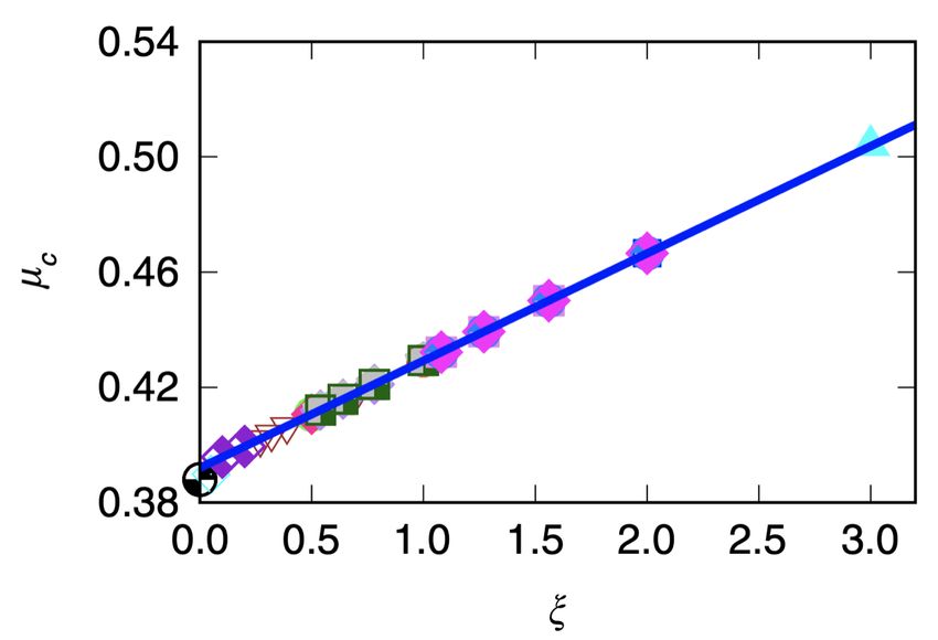
EPJ Web of Conferences 249, 03044 (2021)                                                             https://doi.org/10.1051/epjconf/202124903044
Powders and Grains 2021

                                                                               It can be shown that the value of is 2 in the presence of
                                                                               a saturating liquid and 8/(27Z) ' 0.08 for wet materials.

                                                                               4 Additive rheology
                                                                               We can define a single dimensionless number Im that char-
                                                                               acterizes the perturbation/relaxation process in the pres-
                                                                               ence of the four stresses:
                                                                                                                      !1/2
                                                                                                      tn     1 + /S t
                                                                                                Im = = I                             (14)
                                                                                                      ts      1 + ↵⇠

                                                                               This control parameter should be considered as a gener-
                                                                               alization of the inertial number to cohesive and viscous
                                                                               flows. It contains the inertial, viscous and cohesion num-
                                                                               bers. Hence, the rheology is expected to be fully described
                                                                               by unique functions µ(Im ) and (Im ).
                                                                                   We performed three series of simulations for 1) 2D
      Figure 4. E↵ective friction µ and packing fraction as a func-
      tion of Im in a sheared packing of wet particles simulated for a
                                                                               cohesive-inertial granular flows [6], 2) 2D sheared suspen-
      broad range of parameters. For each set of simulations, the sym-         sions [4], and 3) 3D sheared viscous and cohesive flows
      bols and their colors correspond to the parameters that are varied       [7]. In all cases, for broad range of values of liquid vis-
      with their ranges, all other parameters being kept constant [7].         cosity, cohesion number and inertial number all the fric-
                                                                               tion and pacing fraction data points collapse on a master
                                                                               curve when plotted as a function of Im . Figures 4 and 3
                                                                               show the collapsed data for 3D visco-cohesive flows and
      It should be noted that that the cohesive stress is often de-            2D suspensions. Interestingly, the data are nicely fit by the
      fined by its order of magnitude. For example, for capillary              same functional forms as in dry granular flows, thus unify-
      forces, we may set 0c = ds = fc /(⇡d2 ), where s is the                  ing cohesive and cohesionless granular flows, on the one
      surface tension of the liquid. This di↵ers from the exact                hand, and viscous sheared suspensions and granular flows,
      expression of c given by equation (7). For this reason, in               on the other hand.
      equation (10) ⇠ should be replaced by ↵⇠. Comparing the                      I warmly thank my dear colleagues J.-Y. Delenne and
      two expressions, we get ↵ = 1/(3Z ). In QSFS, we get                     S. Nezamabadi, as well as my ex-students P. Mutabaruka,
      ↵ ' 0.09 by setting Z ' 6 and ' 0.6. Hence,                              L. Amarsid, T.T. Vo and N. Berger for insightful discus-
                                  ⌧                                            sions on the topics presented in this paper. The simulation
                          µc =          = µ(1 + ↵⇠)                 (11)       data were adapted from cited papers.
                                   p

      This is what we observed from 3D simulations of packings
      of spherical particles with capillary forces, as shown in
                                                                               References
      Fig. 2 with ↵ ' 0.09 [7]. The viscous forces may be                      [1] F. Radjai, H. Troadec, S. Roux, Key features of gran-
      either due to the action of a saturating liquid or lubrication               ular plasticity, in Granular Materials: Fundamen-
      forces acting at the gaps between particles in wet granular                  tals and Applications, edited by S. Antony, W. Hoyle,
      materials. The viscous stress is v = ⌘ f ˙ . Using equation                  Y. Ding (RS.C, Cambridge, 2004), pp. 157–184
      (4) and replacing fy by ⌘ f ˙ , we get the corresponding                 [2] GDR-MiDi, Eur. Phys. J. E 14, 341 (2004)
      perturbation time
                                                                               [3] F. Boyer, E. Guazzelli, O. Pouliquen, Phys. Rev. Lett.
                                               !1/2                                107, 18 (2011)
                                         ⇢s
                             tv = d                   .             (12)       [4] L. Amarsid, J.Y. Delenne, P. Mutabaruka, Y. Monerie,
                                        ⌘f ˙                                       F. Perales, F. Radjai, Phys. Rev. E 96, 012901 (2017)
      However, the perturbation time can not be arbitrarily sep-               [5] M. Trulsson, B. Andreotti, P. Claudin, Phys. Rev. Lett.
      arated between the kinetic and viscous e↵ects when both                      109, 118305 (2012)
      e↵ects are simultaneously present. We use again stress ad-               [6] N. Berger, E. Azéma, J.F. Douce, F. Radjai, EPL-
      ditivity to sum the two stresses. As ⌘ f ˙ and ⇢ s d2 ˙ 2 rep-               Europhysics Letters 112 (2015)
      resent only the orders of magnitude of the viscous and                   [7] T. Vo, S. Nezamabadi, P. Mutabaruka, J.Y. Delenne,
      kinetic stresses, we use a linear weighted combination                       F. Radjai, Nature Communications 11, 1 (2020)
        s =    i +   v =   i (1 + /S t), where S t =  i / v is the             [8] F. Radjai, S. Roux, Phys Rev Lett 89, 064302 (2002)
      Stokes number. The perturbation time is given by                         [9] L. Staron, F. Radjai, J. Vilotte, Eur. Phys. J. E 18, 311
                                       !1/2                                        (2005)
                            ⇢s                         ti
             ts = d                           =                 .   (13)
                       i (1 + /S t)               (1 + /S t)1/2

                                                                           4
You can also read