TAMBA: TESTING AND MODELING BRANDEIS ARTIFACTS - dtic.mil

AFRL-RI-RS-TR-2021-002

TAMBA: TESTING AND MODELING BRANDEIS ARTIFACTS

GALOIS, INC.
JANUARY 2021
FINAL TECHNICAL REPORT

 APPROVED FOR PUBLIC RELEASE; DISTRIBUTION UNLIMITED

 STINFO COPY

 AIR FORCE RESEARCH LABORATORY
 INFORMATION DIRECTORATE

 AIR FORCE MATERIEL COMMAND  UNITED STATES AIR FORCE  ROME, NY 13441

NOTICE AND SIGNATURE PAGE

Using Government drawings, specifications, or other data included in this document for any purpose other
than Government procurement does not in any way obligate the U.S. Government. The fact that the
Government formulated or supplied the drawings, specifications, or other data does not license the holder
or any other person or corporation; or convey any rights or permission to manufacture, use, or sell any
patented invention that may relate to them.

This report was cleared for public release by the Defense Advanced Research Projects Agency
(DARPA) Public Release Center and is available to the general public, including foreign nationals.
Copies may be obtained from the Defense Technical Information Center (DTIC) (http://www.dtic.mil).

AFRL-RI-RS-TR-2021-002 HAS BEEN REVIEWED AND IS APPROVED FOR PUBLICATION IN
ACCORDANCE WITH ASSIGNED DISTRIBUTION STATEMENT.

FOR THE CHIEF ENGINEER:

 /S/ /S/
CARL R. THOMAS GREGORY J. HADYNSKI
Work Unit Manager Assistant Technical Advisors
 Computing & Communications Division
 Information Directorate

This report is published in the interest of scientific and technical information exchange, and its publication
does not constitute the Government’s approval or disapproval of its ideas or findings.

Form Approved
 REPORT DOCUMENTATION PAGE OMB No. 0704-0188
The public reporting burden for this collection of information is estimated to average 1 hour per response, including the time for reviewing instructions, searching existing data sources, gathering and
maintaining the data needed, and completing and reviewing the collection of information. Send comments regarding this burden estimate or any other aspect of this collection of information, including
suggestions for reducing this burden, to Department of Defense, Washington Headquarters Services, Directorate for Information Operations and Reports (0704-0188), 1215 Jefferson Davis Highway, Suite
1204, Arlington, VA 22202-4302. Respondents should be aware that notwithstanding any other provision of law, no person shall be subject to any penalty for failing to comply with a collection of information
if it does not display a currently valid OMB control number.
PLEASE DO NOT RETURN YOUR FORM TO THE ABOVE ADDRESS.
1. REPORT DATE (DD-MM-YYYY) 2. REPORT TYPE 3. DATES COVERED (From - To)
 JANUARY 2021 FINAL TECHNICAL REPORT OCT 2015 – APR 2020
4. TITLE AND SUBTITLE 5a. CONTRACT NUMBER
 FA8750-16-C-0022
TAMBA: TESTING AND MODELING BRANDEIS ARTIFACTS
 5b. GRANT NUMBER
 N/A
 5c. PROGRAM ELEMENT NUMBER
 62303E
6. AUTHOR(S) 5d. PROJECT NUMBER
 BRAN
Stephen McGill, Jose Claderon, Benjamin Davis
 5e. TASK NUMBER
 GA
 5f. WORK UNIT NUMBER
 SL
7. PERFORMING ORGANIZATION NAME(S) AND ADDRESS(ES) 8. PERFORMING ORGANIZATION
Galois, Inc. REPORT NUMBER
421 SW 6th Ave, Suite 300
Portland, OR 97204-1622

9. SPONSORING/MONITORING AGENCY NAME(S) AND ADDRESS(ES) 10. SPONSOR/MONITOR'S ACRONYM(S)

Defense Advanced Research Projects Agency AFRL/RITA AFRL/RI
3701 North Fairfax Drive 525 Brooks Road 11. SPONSOR/MONITOR’S REPORT NUMBER
Arlington, VA 22203-1714 Rome, NY 13441-4505
 AFRL-RI-RS-TR-2021-002
12. DISTRIBUTION AVAILABILITY STATEMENT

Approved for Public Release; Distribution Unlimited. DARPA DISTAR CASE # 33505
Date Cleared: 10/14/20
13. SUPPLEMENTARY NOTES

14. ABSTRACT
This report summarizes the TAMBA teams' research and engineering contributions on the DARPA BRANDEIS program.
The focus has been on techniques and technologies for reasoning about privacy. We developed technologies for
measuring the privacy implications and enforcing the privacy guarantees of programs and testing the privacy properties
of databases. Additionally, we developed the theory for modeling the trade-offs between privacy and utitily. We worked
with BRANDEIS technology users to understand and measure end users concerns regarding privacy and privacy
preserving technologies. The program results have been demonstrated through software artifacts and peer reviewed
publications.

15. SUBJECT TERMS

Quantitative Information Flow, Privacy, Information Leakage, Differential Privacy, SQL, Abstract Interpretation

16. SECURITY CLASSIFICATION OF: 17. LIMITATION OF 18. NUMBER 19a. NAME OF RESPONSIBLE PERSON
 ABSTRACT OF PAGES
 CARL R. THOMAS
a. REPORT b. ABSTRACT c. THIS PAGE 19b. TELEPHONE NUMBER (Include area code)
 U U U UU 77 N/A
 Standard Form 298 (Rev. 8-98)
 Prescribed by ANSI Std. Z39.18

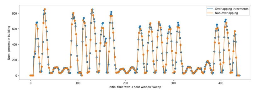
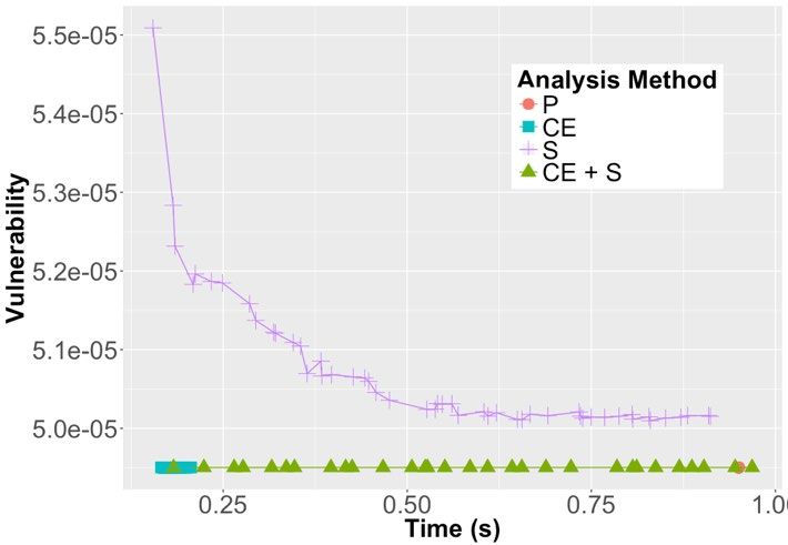
TABLE OF CONTENTS
1.0 Summary ............................................................................................................................. 1
2.0 Introduction ......................................................................................................................... 1
3.0 Methods, Assumptions, and Procedures ............................................................................. 3
3.1 Quantitative Information Flow ........................................................................................... 3
3.1.1 QIF Theory Background ................................................................................................. 3
3.1.2 Deterministic Channels ................................................................................................... 4
3.1.3 Indistinguishability Relation ........................................................................................... 4
3.1.4 The Password Checker Example .................................................................................... 5
3.1.5 Adversary Games ............................................................................................................ 5
3.1.6 Adversary Beliefs and Metrics........................................................................................ 6
3.1.7 Prior Vulnerability .......................................................................................................... 6
3.2 Abstract Interpretation for QIF ........................................................................................... 8
3.3 Model-Counting for QIF ................................................................................................... 11
3.3.1 Computing Static Leakage on Deterministic Programs ................................................ 11
3.4 Bayesian Inference and Privacy ........................................................................................ 12
3.4.1 Prior Model Construction ............................................................................................. 13
3.4.2 Inference ....................................................................................................................... 14
3.5 SQL and Privacy ............................................................................................................... 14
3.6 Information-Flow Control and Liquid Types ................................................................... 14
3.7 Oblivious Computation ..................................................................................................... 15
3.8 IoT and Virtual Sensors .................................................................................................... 16
3.9 Sparse Vector Technique .................................................................................................. 17
3.10 Economic Background ...................................................................................................... 19
3.11 Human Factors and Privacy Controls ............................................................................... 19
3.12 Mental Models for Privacy ............................................................................................... 19
4.0 Results and Discussion ..................................................................................................... 20
4.1 Utilizing prob for analysis of Disaster Response Scenario............................................... 20
4.2 Decomposition-Assisted Scalability ................................................................................. 21
4.3 Improving the scalability of QIF analysis via Sampling and Symbolic Execution .......... 21
4.3.1 Overview ....................................................................................................................... 22
4.3.2 Improving precision with sampling and concolic execution ........................................ 24
4.3.3 Syntax and Semantics ................................................................................................... 26
4.3.4 Computing Vulnerability: Basic procedure .................................................................. 27
4.3.5 Improving precision with sampling .............................................................................. 28
4.3.6 Improving precision with concolic execution ............................................................... 29
4.3.7 Implementation ............................................................................................................. 31
4.3.8 Experiments .................................................................................................................. 32
4.3.9 Conclusions of this work .............................................................................................. 36
4.4 QIF-Supported Workflow Adaptation .............................................................................. 36
4.4.1 HADR Aid Delivery Problem....................................................................................... 36
4.4.2 Scheduling Workflow ................................................................................................... 38
4.4.3 Modeling Workflows .................................................................................................... 39

 i

4.4.4 Supporting Workflow Adaptation................................................................................. 40
4.4.5 Posterior Vulnerability for Steps A+B.......................................................................... 42
4.4.6 Predictive Vulnerability for Step C............................................................................... 42
4.4.7 Posterior Vulnerability for Steps C ............................................................................... 42
4.4.8 Privacy-aware Workflow Adaptation ........................................................................... 43
4.5 Programming Language Enforcement of Privacy............................................................. 45
4.5.1 LWeb............................................................................................................................. 45
4.5.2 A Language for Probabilistically Oblivious Computation ........................................... 45
4.6 Sparse Vector Technique for DP ...................................................................................... 45
4.7 By-hand Analysis of IoT CRT’s Virtual Sensors ............................................................. 46
4.8 Privacy and SQL analysis ................................................................................................. 47
4.8.1 The Relational Scheme Abstract Domain ..................................................................... 48
4.8.2 Per-block Metadata ....................................................................................................... 49
4.8.3 Numeric Abstract Domains in db-priv .......................................................................... 50
4.8.4 Input and Outputs.......................................................................................................... 50
4.8.5 Interactive Weight Revision ......................................................................................... 51
4.8.6 Performance and Optimizations .................................................................................... 51
4.9 Bayesian Evaluations of DP Systems ............................................................................... 52
4.9.1 Deep Learning Approaches to Prior Construction ........................................................ 53
4.10 Equilibrium in Privacy Economics ................................................................................... 57
4.11 Differential Privacy and Privacy Budgets......................................................................... 57
4.12 Modern Data Reconstruction and Other Attacks .............................................................. 58
4.13 User-centered privacy studies ........................................................................................... 60
4.13.1 Virginia Task Force ...................................................................................................... 60
4.13.2 TIPPERS ....................................................................................................................... 60
4.14 Mental Models for End-to-End Encrypted Communications ........................................... 61
4.15 Publications ....................................................................................................................... 62
5.0 Conclusions ....................................................................................................................... 65
6.0 References ......................................................................................................................... 66
7.0 List of Symbols, Abbreviations, and Acronyms ............................................................... 70

 ii

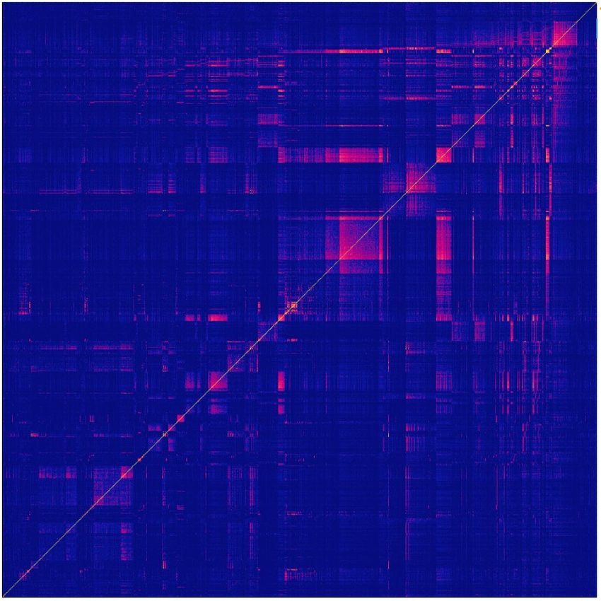
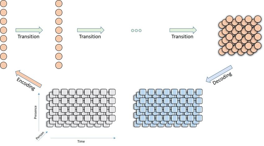
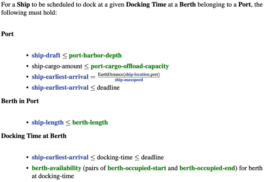
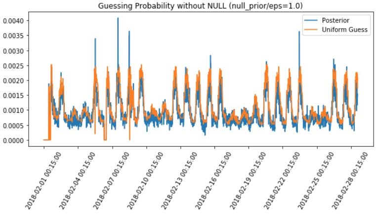
LIST OF FIGURES
Figure 1. The (over)approximation of a polyhedron .................................................................... 10
Figure 2. Numeric Sparse Vector Technique (NSVT) Algorithm ................................................ 18
Figure 3. Prob Encoding of an SQL Query................................................................................... 20
Figure 4. Scalability Improvements with Decomposition ............................................................ 21
Figure 5. Data Model Used in the Evacuation Scenario ............................................................... 23
Figure 6. Algorithm to Solve the Evacuation Problem for a Single Island .................................. 24
Figure 7. Computing Vulnerability (Max Probability) Using Abstract Interpretation ................. 25
Figure 8. Core Language Syntax .................................................................................................. 26
Figure 9. Concolic Semantics ....................................................................................................... 30
Figure 10. Experimental Results ................................................................................................... 34
Figure 11. Constraints in the Scheduling Problem ....................................................................... 37
Figure 12. Predictive Vulnerability of Steps A+B ........................................................................ 41
Figure 13. Posterior Belief over the Position of Ship #9 in the HADR Scenario at Step D ......... 41
Figure 14. Predictive Vulnerability of Step C .............................................................................. 42
Figure 15. Comparison of Initial (Prior) and Post-Task (Posterior) Vulnerability Assessments . 44
Figure 16. Occupancy Algorithm ................................................................................................. 47
Figure 17. A Conceptual Depiction of Factored Particle Filtering (FPF)..................................... 52
Figure 18. Example of the “Guessing” Probability with Factored Particle Filtering ................... 52
Figure 19. Application of the Recurrent Autoencoder Architecture............................................. 53
Figure 20. Bottlenecking Cross-Individual Correlation via Global Features ............................... 54
Figure 21. Time Series Plot of Total Presence in Building .......................................................... 54
Figure 22. Scaled Similarity Matrix.............................................................................................. 55
Figure 23. Transition Matrix with Log Probabilities .................................................................... 56

 LIST OF TABLES
Table 1. Analyzing a 3-ship Resource Allocation Run................................................................. 35
Table 2. Summary of Private Data by Data Owner ...................................................................... 38

 iii

1.0 SUMMARY

In this report we summarize our research and engineering contributions on the Brandeis program.
The focus of our work has been on techniques and technologies for reasoning about privacy.
With this goal in mind, we developed technologies for measuring the privacy implications of
programs, for enforcing the privacy guarantees of programs, for testing the privacy properties of
databases. Additionally, we developed theory for modeling the trade-off between privacy and
utility. We worked with users to gain a better understanding of the end-user concerns regarding
privacy and privacy-preserving technologies. Our results have been demonstrated through a
collection of software artifacts and peer-reviewed research articles.

Our key results include:

• A technique for improving bounds on the results of box-based Quantitative Information
 Flow (QIF) analysis [1]

• A system for analyzing and displaying the possible locations of ships taking part in the
 Coalitions Scenario

• A tool for performing leakage analysis on SCALE-MAMBA programs

• A framework for the analysis of a subset of SQL that supporting the computation of several
 privacy-preserving metrics

• Techniques for using Liquid Types for privacy policy enforcement

• An implementation of the Online Multiplicative Weights algorithm for Differential Privacy

• Organized user-studies for determining how users perceive the privacy/utility trade-off

• Studies of users’ mental models for properties of secure messaging apps and how to
 improve users’ understanding

We discuss each of these accomplishments in detail in this report.

2.0 INTRODUCTION

The TAMBA effort provided new results in both the theoretical and practical aspects of privacy
measurement and reasoning. This range of results includes new scalability techniques for the
analysis of Quantitative Information Flow in programs, as well as work on the human-factors of
privacy. Because of the variety of work done under the TAMBA umbrella, we will describe each
in turn.

Privacy Measurement and Policy Enforcement

In Section 3.1 we provide background on the theory of Quantitative Information Flow (QIF), a
technology that allows for the measurement of privacy leakage. QIF is one of the key theories
that informed a significant portion of TAMBA’s work on Brandeis. The theory of Quantitative

 Approved for Public Release; Distribution Unlimited.
 1

Information Flow can be made into a tool via several implementation strategies. Section 3.2
describes the use of Abstract Interpretation as a method of measuring Quantitative Information
Flow. Another strategy for measuring Quantitative Information Flow, described in Section 3.3, is
to use Model Counting. Section 4.8 describes how the TAMBA team extended some of the
concepts from the prob tool to aid in the analysis of Structured Query Language (SQL), which is
a commonly-used query language in deployed systems and a frequent integration point for
privacy controls.

It is also possible to relate privacy and information leakage to the principles of Bayesian
Inference. This connection is described in Section 3.4 and our research results in this space are
given in Section 4.9. Finally, type systems provide another mechanism for reasoning about and
enforce privacy policies and Section 3.6 describes this research area.

Privacy-Preserving Technologies

We used the tools described above to reason about the privacy properties of systems build atop a
number of privacy-preserving technologies, including differential privacy and secure multi-party
computation. Section 3.7 describes an important aspect of privacy-preserving computation,
Oblivious Computation, which enables computations to be free from standard side-channel leaks.
Section 4.11 describes background on differential privacy. In Section 4.6 we describe a novel
instantiation of the Sparse Vector Technique for differential privacy that incorporates technology
we developed during TAMBA.

The privacy controls above are designed to protect against various privacy attacks. Section 4.12
provides a survey of these attack techniques, which involve various approaches to reconstructing
or de-anonymizing data.

Application Areas

One of the application areas we studied was the Internet of Things (IoT). IoT technology is
increasingly found in homes, buildings, and public spaces. Section 3.8 describes one such system
and Section 4.7 describes the results of our analysis of that system. Section 4.1 describes another
application area we examined: the Enterprise Collaborative Research Team (CRT) Coalitions
Scenario. We describe in that section our process and results for using the prob tool to analyze
Quantitative Information Flow in the Enterprise CRT Coalitions Scenario. This work informed
algorithm changes that preserved more privacy while maintaining the ability to find solutions to
the resource allocation problem. In attempting to scale the analysis along with the increase in
complexity of the Coalitions Scenario, we determined that in some instances Model Counting
performs more efficiently. The use of model counting for the analysis of the Coalitions Scenario
is described in detail in Section 4.4.

Human Factors and Economics

In addition to privacy tools and algorithms, it is important to consider the role of the human in
privacy-aware systems. Users will alter their behavior based on their understanding of privacy
controls, risk, and tradeoffs. It is critical to ensure that the user understands these tradeoffs and to
study what affect the user’s actions have on long-term performance off a privacy-enabled
system. Section 4.14 describes a set of user-studies which aimed to understand users’

 Approved for Public Release; Distribution Unlimited.
 2

understanding of end-to-end encryption, an important privacy control. Section 4.13 describes the
outcome of interviews with subject matter experts from some key application domains targeted
by the Brandeis CRTs. This understanding helped shape scenarios drawn from those domains
and highlighted the core set of user concerns to focus on when doing privacy and utility analysis.
Section 4.11 describes our work on economic systems for setting privacy levels, which leverages
users’ internal preferences regarding risk mitigation and value accrual together with markets to
set fair prices and privacy levels. Section 4.10 describes the surprising outcomes in these models
when we consider user actions and the effect those have on the equilibrium points in these
economic systems.

3.0 METHODS, ASSUMPTIONS, AND PROCEDURES

3.1 Quantitative Information Flow

Consider the function ( ) = 5. Observing the output of does not reveal anything about the
input, . Early work on measuring the amount of information flow focused on the qualitative
approach, one form of which is known as non-interference [2].

In practical systems, it may be difficult, if not impossible, to provide total isolation. In other
systems, you may wish to share some small part of your private data, but you wish to ensure that
your private data as a whole remains private.

A multi-party computation revealing the average of a set of positive integer inputs from various
parties, is an example of a computation that violates non-interference yet also does not fully
reveal the inputs. The output of this averaging computation reveals something about the inputs
(and in some cases quite a lot — if the average is 0 then we can infer that all inputs were 0). QIF
aims to answer the question: how much information do computations such as these actually
reveal about the private inputs?

3.1.1 QIF Theory Background

Information-Theoretic Channels form the basis of the modern formulation of QIF, for this reason
it is worthwhile to formalize the notion of a channel. A channel consists of a triple, ( , , ). 
is the set of inputs to the channel and is the set of outputs from the channel. We say that the
input is private, and the output is public.

 is a | | × | | matrix. Let = { 1 , … , }. Let = { 1 , … , }. Each row of corresponds to
one possible input of the channel. Each column corresponds to one possible output of the
channel. denotes the probability that, if the input to the channel is , the output will be . To
put it another way, if you imagine that is a random variable, = Pr� = | = �. As a
result, in a valid channel matrix, each row must sum to 1, and each cell must be at least 0.

We will often just talk about channels in terms of the matrix itself, and not explicitly write the 
and sets. They can be inferred from the matrix size. In addition, we occasionally refer to
channels as programs.

 Approved for Public Release; Distribution Unlimited.
 3

In addition, we often pun, and use and both as jointly distributed random variables and as
the support of those random variables: ∼ and ∼ ,_ (the distribution over Y’s emitted
from the channel).

3.1.2 Deterministic Channels

A common example of a deterministic channel is based on the game 20 questions. Suppose that
the ‘secret’ is taken from the following set: {mango, carrot, broccoli, rhubarb}. The channel
representation of the question “is it a fruit?”, is as follows:

 Subject = Pr[Fruit| = ] Pr[Vegetable| = ]
 Mango 1 0
 Carrot 0 1
 Broccoli 0 1
 Rhubarb 0 1
 1 0
 0 1
Note that the channel matrix , itself is just � �, without any of the labels on input and
 0 1
 0 1
output.

Because the channel matrix consists only of 0’s and 1’s, we say that the channel is deterministic;
the output is entirely determined based on the input.

With this deterministic channel, the amount of information revealed about the secret varies with
the response to the question. If the answer is “yes”, then the channel has revealed the entirety of
the secret. We know that the secret must be ‘mango’ because it is the only fruit. However, if the
answer is ‘no’ then we have revealed much less about the secret, as it could be any of the
possible vegetables, all we have learned is that the secret is definitely not ‘mango’.

3.1.3 Indistinguishability Relation

Let’s formalize the intuition from above.

Let be a deterministic channel, and let ≈ denote a relation on such that ≈ ⇔ ∀ ∈
 , , = , . That is, ≈ if they go to the same output when run through . Note that the
equivalence classes of ≈ are in one-to-one correspondence with the (non-empty) outputs of .
For example, the equivalence classes of ≈20 questions are {{Mango}, {Carrot,Broccoli,Rhubarb}}.

We call ≈ the indistinguishability relation, since ≈ means that the adversary cannot
distinguish from in the output of the channel.

Intuitively, a program will be more secure if more inputs are indistinguishable (the equivalence
classes are larger). For example, a channel which maps all outputs to the same value reveals no
information in its output, since all the inputs appear identical when viewed through the channel.

 Approved for Public Release; Distribution Unlimited.
 4

3.1.4 The Password Checker Example

Another common deterministic channel is the password checker. The password checker is a
model of a login page. The adversary attempts to guess the password of a single user, and then
gets told whether their guess is correct or incorrect.

The channel is shown below.

 Password = Pr[ = ] Pr[ ≠ ]
 1 0 1
 2 0 1
 ⋮ ⋮ ⋮
 1 0
 ⋮ ⋮ ⋮
 0 1
In other words, given a password guess , we can make a channel that reveals whether the secret
password matches the guessed password.

Note that our experimental model does not consider the generation of an adversary’s public
input. Because of this, models like the above only hold when the possible private values are
drawn from a uniform distribution.

3.1.5 Adversary Games

In the study of QIF it is common to use adversarial games as a method for reasoning about a
given scenario. These provide a way for us to be explicit about how an adversary can behave,
what information it is told, and what constitutes a ‘win’ for that adversary. These games are
played by two players: the defender who is trying to defend the secret data that they input, and
the attacker/adversary who is trying to attack/guess the secret data.

The Prior Game

1. The defender, picks an input, ∈ 

2. The adversary then attempts to guess 

3. The adversary wins if they correctly guess the secret (otherwise, the adversary loses)

Let us consider the twenty questions example once again. One possible way to choose the secret
is uniformly: In this case, we’d say = Uniform( ) = [. 25 . 25 . 25 . 25]. Another
possibility is that, for whatever reason, we are less likely to choose Rhubarb. If an adversary
knows this, they could then assign a lower probability to Rhubarb, and a higher probability to the
other possible subjects. For example: = [. 3 . 3 . 3 . 1].

Formally the prior game is described as follows [3]:

 Approved for Public Release; Distribution Unlimited.
 5

(The notation means that, at this step in the game, the variable is randomly sampled
from the distribution .)

Note that it is incorrect to think of the prior, as what the adversary knows about . is how
the defender chooses ∈ . In this particular game, we are revealing to the adversary. In later
games, the adversary will not be told . In these games, the adversary belief is distinct from the
prior.

Alternatively, you could view as the adversary’s belief about the distribution of , under
assumption that the adversary’s belief is correct.

3.1.6 Adversary Beliefs and Metrics

We are now able to look at various privacy metrics, which are described in terms of adversarial
games. An important concept in these metrics is that of Vulnerability. Vulnerability measures the
probability that the adversary will guess the secret ∈ in one guess.

3.1.7 Prior Vulnerability

The prior vulnerability, which is written as ( ), is defined as the the probability that an optimal
adversary has of winning the prior game.

Two optimal strategies are:

1. Guess sampled from Uniform(argmax ( )), or
 ∈ 

2. Deterministically always guess some element ∈ argmax ( )
 ∈ 

Posterior Game

If prior vulnerability quantifies an adversary’s knowledge prior to seeing the output of a channel,
then the posterior vulnerability quantifies how much an adversary knows after seeing the output
of the channel.

This is modeled by the posterior game [3]:

 Approved for Public Release; Distribution Unlimited.
 6

The defender, picks an input, ∈ . Next, the defender then reveals to the adversary the result
 ∈ of running the input through the channel. Finally, the adversary then attempts to guess .
They win if they correctly guess our secret , and they lose if they do not.

There are two scenarios that we’re going to consider with the posterior game:

Static Scenario

We are attempting to predict, before the channel is run on the concrete secret, how much will be
leaked about the secret. This is called static leakage, or predictive leakage, and we’ll be
introducing it later.

Dynamic Scenario

We have a concrete channel output that is the result of running the channel on some concrete
input. We want to assess how much was leaked by a specific, concrete run of a channel. This
scenario is called dynamic leakage.

In other words, in the static scenario, we want to determine the probability that the adversary will
win the posterior game before step one. In the dynamic scenario, we want to estimate the
probability that the adversary will win after step two (and having seen , but not ).

The two most common vulnerability metrics in the literature are the expected and the worst-case
vulnerabilities.

Expected/Average Posterior Vulnerability

Expected posterior vulnerability is defined as:

 � avg ([ , ]) is the probability that an optimal adversary has of winning the posterior game.

Note that, for the above definition, we only know and . Because we are looking at the static
scenario, we do not have a concrete output value .

Worst-Case Posterior Vulnerability

 Approved for Public Release; Distribution Unlimited.
 7

The worst-case posterior vulnerability, is � worst ([ , ]) is the worst conditional vulnerability
which might be achieved by any output.

 � worst ([ , ]) = max⌈ | ⌉
 = max ( | )
 ∈ 
 = max Pr[ = | = ]
 ∈ , ∈ 

Worst-Case vs Expected Posterior Vulnerability

The key difference between worst-case and expected posterior vulnerability is that worst-case
posterior vulnerability does not take into account how unlikely a particular input may be, only
how much it might reveal about the private data.

This is most evident in the password checker example, suppose there are 2256 possible
passwords. Then, with high probability, the channel will not reveal the secret, and leakage will
be small. There is a very small probability that the channel will reveal to the adversary the entire
password. Therefore, the worst-case vulnerability is 1 for the password checker, despite it being
very unlikely that it would reveal the password.

The expected posterior vulnerability will weigh each outcome according to how likely it is, and
will therefore report a lower vulnerability than the worst-case metric.

3.2 Abstract Interpretation for QIF

Abstract interpretation is a technique for making tractable the verification of otherwise
intractable program properties [4]. As the term implies, abstraction is its main principle: instead
of reasoning about potentially large sets of program states and behaviors, we abstract them and
reason in terms of their abstract properties. We begin by describing the two principal aspects of
abstract interpretation in general: an abstract domain and abstract semantics over that domain.

Abstract Domain:

Given a set of concrete objects an abstract domain is a set of corresponding abstract
elements as defined by two functions:

• an abstraction function : → , mapping sets of concrete elements to abstract elements,
 and

• a concretization function : → , mapping abstract elements to sets of concrete
 elements.

 will be instantiated to either program states or distributions over program states. In
either case, we assume the standard concrete semantics of a simple imperative programming
language, Imp. Because you can view a program’s state as a point in a multidimensional space,
we often refer specific sets or distributions of program states as regions.

 Approved for Public Release; Distribution Unlimited.
 8

For convenience we will consider abstract domains that can be defined as predicates over
concrete states. I.e., : ↦ { ∈ : ( )} where is a predicate parameterized by the abstract
element .

The second aspect of abstract interpretation is the interpretation part: an abstract semantics,
written ⟨⟨ ⟩⟩: → . We require that the abstract semantics be sound in that it over-
approximates the concrete semantics.

Definition 1 (Sound Abstraction): Given an abstract domain and its abstract semantics, the
abstraction is sound if whenever ∈ ( ) then [[ ]] ∈ (⟨⟨ ⟩⟩ ).

Abstractions generally sacrifice some precision: the abstraction of a set of elements can be
imprecise in that ( ( )) contains strictly more than just and likewise that (⟨⟨ ⟩⟩ )
contains strictly more elements than {[[ ]] : ∈ ( )}. For this reason, an analysis
satisfying Definition 1 is called a may analysis in that it contains the set of all states that may
arise during program execution.

Numeric Abstractions

A large class of abstractions are designed specifically to model numeric values; in this chapter
we restrict ourselves to integer-valued variables. The interval domain represents “boxes” or
non-relational bounded ranges of values for each variable in a state [5]:

 : {( , )} ↦ { ∈ : ≤ ( ) ≤ for every }

Abstract elements here are sets of bound pairs, and , forming the lower and upper bound,
respectively, for every variable . Intervals are efficient to compute, but imprecise, in that they
cannot characterize invariants among variables. More precise, but less efficient numeric domains
can be used.

More generally, an abstract domain can be defined in terms of a set of predicates over states,
interpreted conjunctively:

 : � � ↦ � ∈ : ( ) for every �

Restrictions on the types of predicates allowed define a family of abstractions. Examples include
intervals already mentioned, polyhedra ℙ where are restricted to linear inequalities, and
octagons [6] where the linear inequality coefficients are further restricted to the set {−1,0,1}.
Polyhedra and octagons are relational in that they allow precise representations of states that
constrain variables in terms of other variables (note this is not the case for intervals). In terms of
tractability, intervals are faster to compute with than octagons which are faster than polyhedra.
Precision follows the reverse ordering: polyhedra are more precise than octagons which are more
precise than intervals. In other words, intervals can over-approximate the set of points
represented by octagons which themselves can over-approximate the set of points represented by

 Approved for Public Release; Distribution Unlimited.
 9

polyhedra. This relationship is visualized in Figure 1, which shows the (over)approximation of a
polyhedron (black) using an octagon (shaded, left) and an interval (shaded, right).

 Figure 1. The (over)approximation of a polyhedron
Abstract domains implement a set of standard operations including:

• Meet, ⊓ is the smallest region containing the set of states in the intersection of
 ( ), ( ). For convex linear domains this operation is least expensive and is exact.

• Join, ⊔ is the smallest region containing both ( ) and ( ). For linear convex
 domains, this is supported by the convex hull operation.

• Transform, [ → ], computes an over-approximation of the state-wise assignment ↦
 . In the case of invertible assignments, this operation is supported by linear domains via
 affine transformation. Non-invertible assignments require special consideration [7].

Abstraction combinators

Abstractions can also be extended disjunctively as in the powerset construction [8]. For a base
domain , the powerset domain has concretization:

 : � � ↦ � ∈ : ∈ � � for some � =∪ � �
 
That is, an abstract element in is itself a set of base elements from and represents the set of
states represented by at least one of its constituents’ base elements.

Abstraction in the manner outlined can also be applied to probability distributions which serve as
the concrete elements. Earlier techniques [9] attached probability constraints to standard state
domains. Given a state domain we form the probabilistic (upper bound) domain ( ) that
adds a probability bound on all states represented by the base domain elements:

 : ( , ) ↦ { ∈ : ( ) ≤ for all ∈ ( )}

We can combine the probabilistic upper bound construction the powerset construction to define a
domain for representing more complex distributions. A more expressive variant of powerset for
probabilistic abstractions imposes a sum bound (as opposed to disjunction of bounds):

 Approved for Public Release; Distribution Unlimited.
 10

 : �( , )� ↦ � ∈ : ( ) ≤ � for every �
 : ∈ ( )

We emphasize in these abstractions the focus on the upper bounds of probability; such
abstractions do not explicitly track lower bounds (beyond the assumed trivial 0). That is, for any
probabilistic abstraction and any state , there exists ∈ ( ) such that ( ) = 0.
Because of this, these upper bound abstractions lack sound definitions of conditioning.

3.3 Model-Counting for QIF

Boolean SATisfiability problem (SAT) and Satisfiability Modulo Theories (SMT) solvers
provide a method for users to solve a decision problem and determine whether or not there exists
a solution which satisfies some constraints. A model counter is able to take the same set of
constraints and determine the number of possible solutions which satisfy them. For the SAT
decision problem, the analogue model counting problem is #SAT (pronounced “sharp-SAT”),
and for SMT it is #SMT.

3.3.1 Computing Static Leakage on Deterministic Programs

Recall that, the min-capacity of a deterministic channel is the base-2 log of its number of
(feasible) outputs [3]. This result allows us to use model counters as a method to computer the
min-capacity. Importantly, because many existing program verification techniques require the
conversion of source code to a formal model (that can be passed to an SMT solver or similar),
#SAT approaches to computing min-capacity can leverage this existing technology to operate on
actual programs.

Biondi et. al. [10] describe the general approach:

1. Convert a program to a SAT formula

2. (Approximately) count the number of satisfying assignments of the output variables 1

3. Return the base-2 log of this count.

Biondi et. al. [10] use the CBMC model checker to convert C code to a formula, and then they
use ApproxMC2 model counter to count the number of outputs.

Backes et. al. [11] use a different approach. They iteratively refine an indistinguishability
relation until it matches the program they want to analyze. Starting with a partition which
contains all outputs in a single bin, they use a SAT solver to prove or disprove whether it is
possible to distinguish between two inputs in the same bin. If it is disproven, then the algorithm
terminates. Otherwise, they split a bin in the partition and then step again.

1
 Because both input and output variables will be constrained by the formula, we need to be
careful to only count the number of outputs.

 Approved for Public Release; Distribution Unlimited.
 11

3.4 Bayesian Inference and Privacy

In the course of the latter parts of the TAMBA effort, the Charles River Analytics (CRA) team
has focused on developing empirical evaluations of privacy systems based on Bayesian
probability theory. We’ve focused in particular on methods to attack and utilize differential
privacy (DP) systems via Bayesian inference. Differential privacy systems provide a precise
mathematical guarantee – the practical significance of which is unclear (and sometimes
overstated):

 Pr( ( 1 ) ∨ 1 ) ≤ Pr( ( 2 ) ∨ 2 )∀ 2 ∈ Adj( 1 )

That is, the conditional probability of some -differentially private algorithm output given an
input dataset 1 is bounded by a factor of from all other datasets Adj( 1 ) adjacent to 1 .
Adjacency can be freely defined by the system developer. Often it is defined as single
perturbations to a dataset – the addition or removal of a single individual from a database, for
instance.

This definition alone does not define pragmatic privacy guarantees, however, as one is really
interested in the probability of the underlying data given the output of the DP algorithm.
Applying Bayes rule:

 Pr( 1 )
 Pr� 1 ∨ ( 1 )� ≤ Pr� 2 ∨ ( 2 )� ∀ ∈ Adj( 1 )
 Pr( 2 ) 2

The posterior probability of a given dataset is thus additionally related to the relative prior
probabilities of adjacent datasets. When this ratio of prior probabilities is far from 1 there can be
significant venue for adversarial reconstruction – potentially arbitrarily far from the promises of
differential privacy. Common circumstances can induce this – for instance, we spent significant
analysis time on a person localization dataset constructed by the University of California, Irvine
(UCI) IoT CRT team. If one defined adjacency as the addition or removal of an individual from a
single detection in a building on 5-minute increments, this would contradict most prior models.
A dataset in which an individual sits in their office for 30 minutes, disappears for 5 minutes, and
then reappears in their office for 30 minutes would be highly unlikely according to reasonable
 Pr( 1 )
prior models. Thus could be very large – potentially as high as 100 or 1000 (or 1e-2 / 1e-3,
 Pr( 2 )
equivalently).

One of our major goals in the Brandeis program was also to provide an effective utility-based
analysis of DP systems. This, likewise, benefits greatly from strong inference capabilities. In
general, a user might be interested in the posterior distribution of some function – for instance,
one might want to know the distribution of possible individuals in a room (as a direct application
of the DP system). Likewise, for evaluating a DP system, one might want to evaluate the
accuracy of localizing individuals and demonstrate that it is not possible with high accuracy.
Both of these cases are answered correctly and completely by posterior evaluation of the
distribution of interest given DP output – that is:

 Pr� | ( 1 )� = ∫ 1 Pr( ∨ 1 )Pr� 1 | ( 1 )�

 Approved for Public Release; Distribution Unlimited.
 12

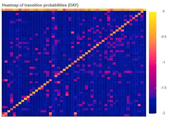
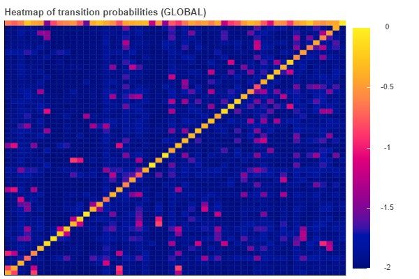
One might also be interested in amortizing over the actual execution of the DP system – to
understand, for instance, the typical range of various metrics. This is also naturally stated as
Bayesian inference:

 Pr( | 1 ) = ∫ 1′ Pr( | 1′ )∫ ( 1 )Pr� 1 ′| ( 1 )�Pr( ( 1 ) ∨ 1 )

In this case the formula describes typical inferred values for metric given a ground-truth
dataset 1 .

3.4.1 Prior Model Construction

There are two challenges associated with casting DP evaluation as a Bayesian inference problem.
First, one must construct a prior model ( ) describing what datasets are “reasonable”. There
are a number of approaches to this, a number of which were explored under this effort. A popular
technique would be to employ one of a number of classical approaches to distribution
construction that have nice mathematical properties. Our first explorations involved the
construction of Markov models describing person movement. These models made two
assumptions that are highly dubious, however, and inhibit realistic analysis. First, in the UCI
dataset context, we assumed individuals moved independently. Second, we assumed that the
most recent location of an individual fully described the system “state” – that is, the prediction of
future movement could not be made more accurate by also accounting for older location
information. These models could be refined from data, fortunately, and the single room-to-room
transition matrix that defines that Markov model was estimated from the UCI dataset.

A second approach we explored was the application of deep neural networks (DNNs) to learn
hidden Markov models describing the datasets. These learned HMMs could capture complex
temporal and cross-individual information from available data, though they presented some
challenges. Training these models is computationally onerous and practically difficult due to
strong biases in the data. Furthermore, evaluating these models can be highly ambiguous –
serious thought about cross-validation must be employed to determine if metric inference is due
to a sophisticated “general” prior regarding person movement or if instead one has learned a
model that memorized certain attributes. It can be difficult to ascertain if the model has
memorized a class schedule or a given individual’s office location, for instance. This is a critical
point because one would like to employ these priors to evaluate DP algorithms under reasonable
adversary models – priors leveraging strong machine learning can capture some of the optimal
structure a domain expert might be capable of articulating, but they also might be unreasonably
strong due to their application of data an adversary would not have access to.

The third, most general approach we explored was the construction of prior distributions based
on probabilistic programs. Probabilistic programming provides a flexible architecture for
constructing probability distributions using programming language constructs – for instance, one
can use object-oriented approaches to describe entities such as Person, Meeting, or Office that
capture the semantics of the domain of interest. These entities can then be related via a variety of
probabilistic models, varying from simple models like the Markov models described above to
complex models like those described by DNNs. By embedding the domain semantics in the
model, it is possible to both capture the domain expertise in a manner an adversary might be

 Approved for Public Release; Distribution Unlimited.
 13

capable of as well as learn parameters related to the semantics of the domain rather than a black-
box relation – this greatly reduces training data requirements and enhances generalization.

3.4.2 Inference

Given a prior model, the next challenge is performing probabilistic inference – that is,
calculating Bayes rule variable posteriors given observations from a DP system. General
inference is known to be intractable – in essence, one must calculate a number of integrals over a
high dimensional space. There exist a number of feasible approaches for special cases, but only
approaches under development now are capable of providing useful results for the more general
problem settings we are interested in, e.g. for probabilistic program models. In the later sections
we will describe our approaches to inference. Further advancement in the field of tractable
inference on more complex models will make these analyses more feasible in the future.

3.5 SQL and Privacy

There is a significant amount of work on SQL implementations and tools that enable privacy-
preserving database usage. Differential Privacy provides a theoretical framework for the study
and development of privacy preserving mechanisms in query-based data analysis (such as SQL).
Work such as McSherry’s Privacy Integrated Queries (PINQ) [12] provides programmers with
the advantages of differential privacy in familiar contexts. However, differential privacy does not
provide a framework for discussing the amount of information that is revealed in a set of queries.
This sort of reasoning requires an analysis of the SQL queries in question, and would be useful
even in the case where no differentially private mechanism is used or desired in a system.

Work on the analysis of SQL queries has focused on more conventional concerns of database
users, analysts, and administrators: performance, change impact prediction, type errors [13].
Many researchers have also investigated the use of static analysis of SQL for detecting security
issues [14], [15].

3.6 Information-Flow Control and Liquid Types

There is a significant amount of work in Information-Flow Control (IFC) and type systems that
enforce information-flow policies [16]. This work differs from QIF in that IFC analyses do not
quantify how much information regarding the secret data has flowed (or leaked) to the output, but
whether any information flow has occurred. This reduction in ambiguity allows for more
tractable analysis and enforcement, at the cost of being able to quantify the risk of running a
particular program.

Information-flow policies often deal with various forms of declassification along four axes: who,
what, where, and when. Who determines which actors are able to receive declassified
information. What determines what data is able to be declassified. Where determines what
subsets of data can be declassified. When is used for when secret data is only sensitive for a
certain period of time.

Static type systems are an attractive avenue for enforcing IFC policies for a few reasons:

 Approved for Public Release; Distribution Unlimited.
 14

• Runtime/dynamic analyses cannot observe all possible paths of the computation, allowing
 for the program to correctly enforce the policy in some instances and not in other. This
 means that any failure at runtime due to policy enforcement reveals the fact that secret
 information was going to flow to the output.

• External static analyses require the programmer to be judicious in the use and application of
 the static analysis tool itself. There is no guarantee that the results of any static analysis will
 be incorporated into the program in question.

• Type systems enforce the policies intrinsically: the program cannot be run or compiled if
 the program does not pass the static type-checker. This also gives confidence to the
 developer by guaranteeing that a compiled program is safe with regards to the information-
 flow policies.

One solution to these problems is embodied in the Labeled IO (LIO) system [17] for Haskell.
LIO is a drop-in replacement for the Haskell IO monad, extending IO with an internal current
label and clearance label. Such labels are lattice ordered (as is typical [18]), with the degenerate
case being a secret (high) label and public (low) one. LIO’s current label constitutes the least
upper bound of the security labels of all values read during the current computation. Effectful
operations such as reading/writing from stable storage, or communicating with other processes,
are checked against the current label. If the operation’s security label (e.g., that on a channel
being written to) is lower than the current label, then the operation is rejected as potentially
insecure. The clearance serves as an upper bound that the current label may never cross, even
prior to performing any I/O, so as to reduce the chance of side channels. Haskell’s clear, type-
enforced separation of pure computation from effects makes LIO easy to implement soundly and
efficiently, compared to other dynamic enforcement mechanisms.

3.7 Oblivious Computation

An ‘oblivious computation’ is any computation that is free from information leaks which are due
to observable differences in the timing of the computation or in the memory-access patterns of
the computation. Oblivious programming languages offer mechanisms for ensuring that all
programs written in the language are oblivious by construction. For example, in a traditional
programming language the if construct is a source of potential side-channels, consider the
following:
 if (p) {
 
 } else {
 
 }

In the instance where stmts1 and stmts2 are not identical (the common case, as otherwise the
conditional branching is unnecessary), it may be possible for a third-party to determine p’s value
based purely on external observations, such as knowing that stmts2 is a significantly more
expensive computation. If p is meant to be secret, this is a significant issue, rendering the
computation not oblivious. One method of making the above oblivious is by ensuring that
regardless of p’s value, both branches are executed, i.e. all of stmts1 and stmts2 are processed,

 Approved for Public Release; Distribution Unlimited.
 15

but only the results from the semantically necessary branch are used. This ensures that no side-
channel information is leaked regarding the value of p. However, this also means that the
programming environment must manage side-effects carefully. Consider the following:
 ...

 if (p) {
 a = x + y;
 } else {
 a = x + z;
 }

 return a;

Attempting to execute the above in an oblivious manner raises the question “what should be
returned as a’s value?” This can be addressed via several means, having effects that can be
‘rolled back’, or forbidding side-effects such as assignment or mutation.

3.8 IoT and Virtual Sensors

The increasing use and presence of Internet of Things (IoT) devices has led to privacy concerns
for both the consumer of the IoT devices and for people in public spaces. The TIPPERS project,
at The University of California, Irvine, is a smart-building developed, in part, to study the
privacy implications of IoT devices and their use in a working environment [19]. The TIPPERS
system is deployed in the Bren Hall on the UC Irvine campus. The building provides IoT devices
that monitor various aspects of the daily use of the building: HVAC, lighting, occupancy, access
control, CCTV, and so on. TIPPERS abstracts over these systems and aims to provide privacy-
aware querying and analysis of the system data [19].

One such privacy-aware abstraction over the raw IoT systems are an abstraction named
SemIoTic, which provides a set of ‘virtual sensors’ [20]. These virtual sensors aim to provide
smart-building application developers with tools for determining high-level building information
(occupancy, temperature, energy usage, etc.) without providing access to the raw sensor data,
which may (intentionally or not) violate privacy requirements. For example, the raw WiFi
access-point data could be used to estimate room occupancy, but that very same data (MAC
address connection and disconnect events) can be easily tied to a particular individual [20].

SemIoTic virtual sensors also perform some computation on the raw sensor data in order to
provide more meaningful semantic information to the developer. One example of such a
computation is occupancy estimation. If an individual’s WiFi enabled device connects to an
access point that is near, but not in, their office, the virtual sensor code will rate their presence as
being more likely to be in their office.

 Approved for Public Release; Distribution Unlimited.
 16