The Impact of Rising Oil Prices on U.S. Inflation and Inflation Expectations in 2020-23
←
→
Page content transcription
If your browser does not render page correctly, please read the page content below
The Impact of Rising Oil Prices on
     U.S. Inflation and Inflation
      Expectations in 2020-23

                               Lutz Kilian and Xiaoqing Zhou

Working Paper 2116                                                                    November 2021
Research Department
https://doi.org/10.24149/wp2116
Working papers from the Federal Reserve Bank of Dallas are preliminary drafts circulated for professional comment.
The views in this paper are those of the authors and do not necessarily reflect the views of the Federal Reserve Bank
of Dallas or the Federal Reserve System. Any errors or omissions are the responsibility of the authors.
The Impact of Rising Oil Prices on U.S. Inflation and Inflation
                      Expectations in 2020-23*

                                         Lutz Kilian† and Xiaoqing Zhou‡

                                                 November 1, 2021

                                                       Abstract

Predictions of oil prices reaching $100 per barrel during the winter of 2021/22 have raised
fears of persistently high inflation and rising inflation expectations for years to come. We
show that these concerns have been overstated. A $100 oil scenario of the type discussed
by many observers, would only briefly raise monthly headline inflation, before fading rather
quickly. However, the short-run effects on headline inflation would be sizable. For
example, on a year-over-year basis, headline PCE inflation would increase by 1.8
percentage points at the end of 2021 under this scenario, but only by 0.4 percentage
points at the end of 2022. In contrast, the impact on measures of core inflation such as
trimmed mean PCE inflation is only 0.4 and 0.3 percentage points in 2021 and 2022,
respectively. These estimates already account for any increases in inflation expectations
under the scenario. The peak response of the 1-year household inflation expectation
would be 1.2 percentage points, while that of the 5-year expectation would be 0.2
percentage points.

JEL code: E31, E52, Q43

Keywords: Scenario, inflation, expectation, oil price, gasoline price, household survey,
core, pandemic, recovery.

*
 The views in this paper are solely the responsibility of the authors and should not be interpreted as reflecting the views of
the Federal Reserve Bank of Dallas or the Federal Reserve System. We thank Jim Dolmas and Marc Giannoni for helpful
comments. The authors have no conflict of interest to disclose.
†
 Correspondence to: Lutz Kilian, Federal Reserve Bank of Dallas, Research Department, 2200 N. Pearl St., Dallas, TX
75201, USA and CEPR. E-mail: lkilian2019@gmail.com.
‡
Xiaoqing Zhou, Federal Reserve Bank of Dallas, Research Department, 2200 N. Pearl St., Dallas, TX 75201, USA. E-mail:
xqzhou3@gmail.com.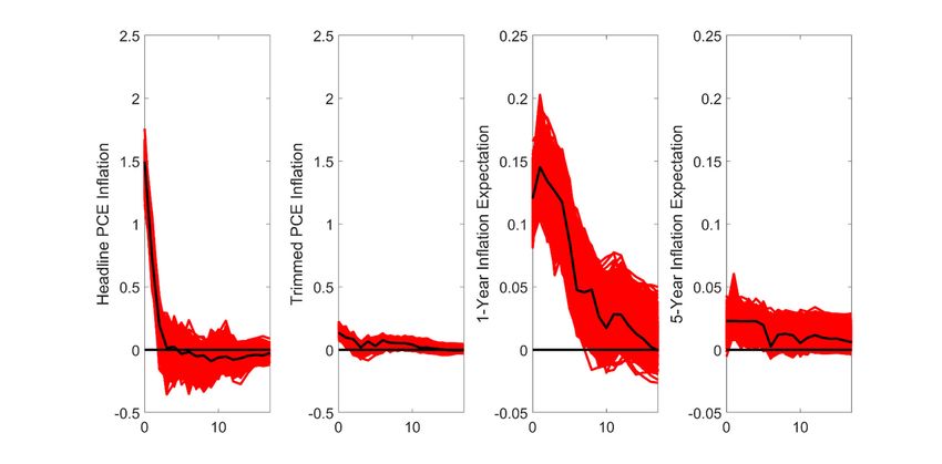
1. Introduction

The surge in inflation rates in 2021 reflected rising demand, as the economy adapted to the

COVID-19 pandemic, tight labor markets, supply chain disruptions and the recovery of

energy prices from their pandemic lows. With the price of West Texas Intermediate (WTI) oil

rising above $80/barrel in October 2021, concerns have grown that the oil price may climb as

a high as $100/in the coming winter, as power plants in Europe and Asia switch to petroleum

products in response to a shortage of coal and natural gas. Such a surge in oil demand

combined with low oil inventories, inadequate oil production in OPEC+ countries and anemic

growth in U.S. shale oil production could push the oil price to levels not seen since the early

2010s.

         There are growing worries among policymakers and analysts that further, substantial

oil price increases could push U.S. inflation higher for extended periods as well as drive up

consumers’ inflation expectations, as rising oil prices are reflected in retail gasoline prices.

This could lead to inflation expectations becoming embedded in the wage and price setting

process. For example, analysts at the Bank of America warned on October 1, 2021, that oil

could surge above $100 in the event of a cold winter and spark inflation (see Lee 2021). This

sentiment is common on Wall Street. Similar views have been expressed by other investment

banks including Goldman Sachs, JP Morgan and Barclay. Likewise, BlackRock, the world's

top asset manager, recently stated that there is a high probability of oil hitting $100 a barrel.

Despite these warnings, there has been no quantitative analysis of this scenario.

         These concerns prompt two key questions. First, to what extent have shocks to the

gasoline price affected U.S. inflation and inflation expectations since the beginning of the

pandemic? Second, how much further would a rise in the price of oil to $100 in the winter of

2021/22 increase inflation and inflation expectations and how persistent would these effects

be over the next two years? The latter question is closely related to the former, since what

                                                 1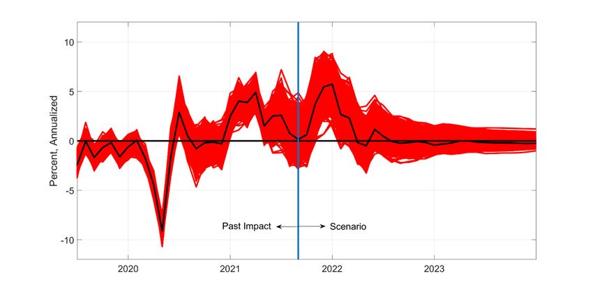
matters to policymakers is the combined cumulative effect on inflation of gasoline price

shocks that have already occurred and gasoline price shocks that are expected to occur, if the

price of oil reaches $100 per barrel in the coming winter.

       We address these questions based on a structural vector autoregressive (VAR) model

of the relationship between nominal retail gasoline prices, headline inflation, core inflation,

and the Michigan Survey of Consumers median 1-year and 5-year inflation expectations. This

model recognizes that it is gasoline prices rather than the price of crude oil that enter the

consumer basket and that the gasoline price is what matters for the determination of

household inflation expectations because of its salience (see, e.g., Coibion and

Gorodnichenko 2015; Binder 2018). The identification of the model builds on insights in

Kilian and Zhou (2021), who show that a structural VAR model is a more natural framework

to estimate the effect of gasoline price shocks on inflation and inflation expectations than

reduced-form correlations. In this paper, we take the analysis a step further by discussing how

scenarios about the future evolution of the price of crude oil (such as the scenario entertained

by the Bank of America) may be econometrically evaluated within our structural VAR

model, along with the impact of past gasoline price shocks on inflation and inflation

expectations.

       We first show that gasoline price shocks account for much of the sharp temporary

decline in headline inflation early in the COVID-19 pandemic. Gasoline price shocks started

creating systematic inflationary pressures in early 2021, but, by September 2021, the

cumulative impact of these gasoline price shocks had greatly diminished, indicating that

much of the continued surge in core inflation and headline inflation at that point was driven

by upward pressure on the prices of other goods. This suggests that the broad-based price

increases from, for example, durable goods (vehicles, furniture, consumer electronics),

shelter (rent and owners’ equivalent rent) and other services (such as medical care) will be

                                                2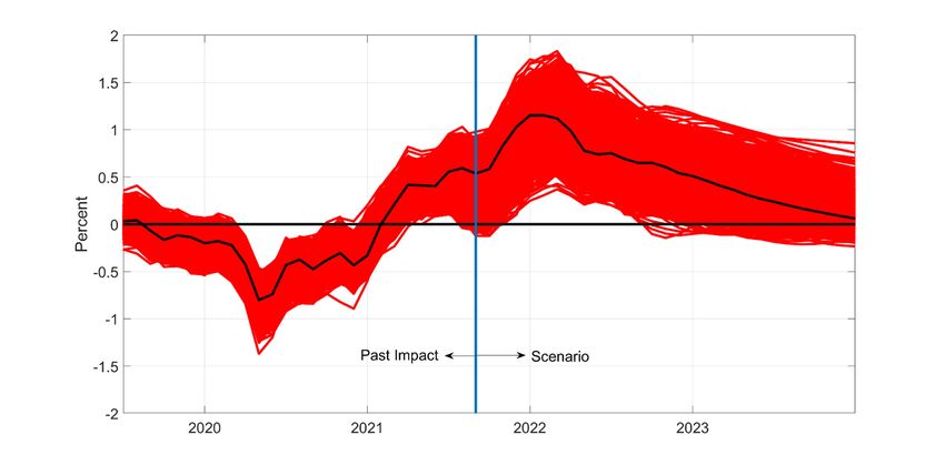
the main drivers of inflation in the years to come. These pressures are likely to persist, even if

oil and gasoline prices were to stabilize at current levels.

       We then examine how renewed gasoline price increases after September 2021 in

response to the oil price reaching $100 per barrel in the winter of 2021/22, as conjectured by

many market observers, would affect inflation and inflation expectations. We show that

concerns about persistently high headline inflation in 2022 and 2023 in response to this

scenario have been overstated. A $100 oil scenario would only briefly raise monthly headline

inflation, before fading rather quickly. However, the short-run effects on headline inflation

would be sizable.

       The precise magnitude of the impact on inflation differs depending on whether we

focus on CPI or PCE headline inflation. On a year-over-year basis, under the $100 oil

scenario, headline CPI inflation would increase by an additional 3 percentage points by the

end of 2021, but headline PCE inflation only by 1.8 percentage points. By the end of 2022,

the impact would drop to 0.4 percentage points for either inflation measure. By 2023, the

effect would be effectively zero. By comparison, core CPI inflation and trimmed mean PCE

inflation measures suggest a much more modest impact. On a year-over-year basis, they

would rise by 0.5 and 0.3 percentage points at the end of 2021, respectively, and by 0.4

percentage points for either measure at the end of 2022.

       All these estimates already incorporate the effect higher gasoline prices may have on

inflation expectations. We find that under the scenario the cumulative effect of gasoline price

shocks on 1-year inflation expectations rises to 1.2 percentage points in late 2021, before

gradually declining. The effect on 5-year inflation expectations is much smaller with a peak

increase of only 0.2 percentage points, suggesting that 5-year household inflation are hardly

affected by gasoline price shocks.

       Our work relates to a large literature on how household survey inflation expectations

                                                 3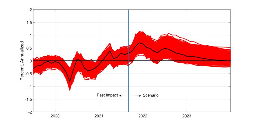
respond to oil and gasoline price shocks (see, e.g., Coibion and Gorodnichenko 2015; Wong
2015; Binder 2018; Conflitti and Cristadoro 2018; Binder and Makridis 2021; Kilian and
Zhou 2021). In addition, our analysis is related to earlier empirical work on how oil and
gasoline price shocks are transmitted to inflation (see, e.g., Kilian 2009; Clark and Terry
2010; Kilian and Lewis 2011; Wong 2015; Conflitti and Luciani 2019; Kilian and Zhou
2021). Our analysis differs from this earlier literature not only in that we are the first to
examine the major fluctuations in inflation and inflation expectations during the COVID-19
pandemic. We also go beyond quantifying inflationary effects in the historical data and show
how to evaluate hypothetical scenarios for the future evolution of oil and gasoline prices and
their impact on inflation and inflation expectations. Moreover, we consider both short-term
and long-term household inflation expectations and we report results for a range of
alternative inflation measures of interest to policymakers rather than just monthly headline
inflation.
The remainder of the paper is organized as follows. In section 2, we introduce a
structural VAR model that allows us to answer the questions of interest under minimal
assumptions and we discuss the econometric tools required for the analysis of scenarios.
Section 3 reports results for the CPI inflation measures most commonly discussed in the press
and for household inflation expectations. Section 4 reports the corresponding results for the
PCE inflation measures favored by central bankers. Section 5 examines the implications of
our estimates for year-over-year inflation rates. The concluding remarks are in Section 6.
2. The Structural VAR Model
Let yt [pgast , t , core t , t1 yr exp , t5 yr exp ], where pgast denotes the growth rate of the
nominal U.S. retail price for unleaded gasoline, t is the headline inflation rate, core t is a
measure of core inflation, and t1 yr exp and t5 yr exp are the Michigan Survey of Consumers’
4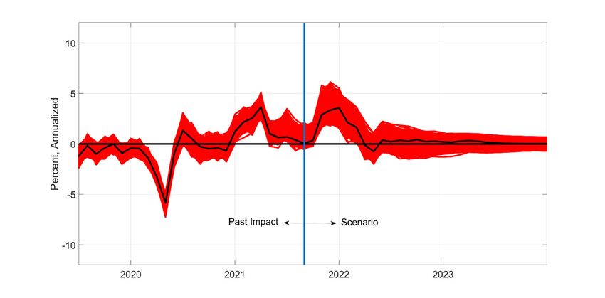
measure of the median household expectation of inflation over the next year and the next five
years, respectively. We postulate that these data are jointly explained by a structural VAR
model. We consider two variants of the model. One is based on headline CPI inflation and
inflation in the CPI excluding food and energy, as a measure of core inflation. The other is
based on headline PCE inflation and the trimmed mean of PCE inflation as the measure of
core inflation. We also selectively report additional results for core PCE inflation. All
variables are measured in percent (see Figure 1).1
2.1. Model structure
The structural VAR model can be written as B0 yt B1 yt 1 ... B p yt p wt , where yt is the
5 1 vector of date t observations for t p 1,..., T , wt denotes the vector of mutually
uncorrelated i.i.d. structural shocks and Bi , i 0,..., p, represent 5 5 dimensional
coefficient matrices. The intercept has been dropped for expository purposes. The reduced-
form VAR model representation is yt A1 yt 1 .... Ap yt p ut , where Ai B01 Bi , i 1,..., p,
and ut B01wt . We set the lag order, p, to a conservative upper bound of 12 lags (see Kilian
and Lütkepohl 2017). The model explains variation in the data in terms of the structural
shocks wt . The model is partially identified in that only the first structural shock is identified.
The estimates of the responses to this shock are invariant to the identification of the
remaining structural shocks (see Christiano, Eichenbaum and Evans 1999).
The gasoline price shock is identified based on the assumption that the nominal price
of gasoline is predetermined with respect to the other model variables. This assumption is
supported by empirical evidence in Kilian and Vega (2011). Under our identifying
assumption
1
The CPI and PCE data are available in FRED. The gasoline price data were obtained from the U.S. Energy
Administration’s Monthly Energy Review. The inflation expectations data were downloaded directly from the
website of the Survey Research Center at the University of Michigan.
5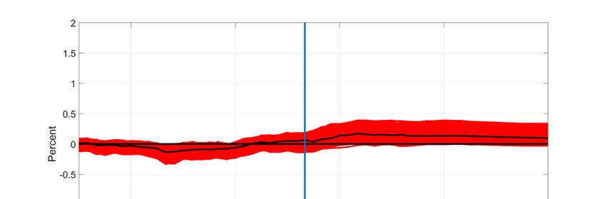
utpgas
CPI * 0 0 0 0 wtnominal gasoline price
*
ut * * * * wt2
core CPI
* * * * * 3
ut wt (1)
1 yr exp *
* * * * wt4
ut
u 5 yr exp * * * * * wt 5
t
and
utpgas
* 0 0 0 0 wtnominal gasoline price
*
* * * *
PCE
ut wt2
trimmed mean PCE
ut * * * * * wt3 . (2)
*
1 yr exp * * * * wt4
ut
u 5 yr exp *
* * * * wt 5
t
The use of a partially identified model not only dispenses with the need for potentially
controversial additional identifying assumptions, but also facilitates the construction of
scenarios for the identified shock. Models (1) and (2) are an extension of a lower-dimensional
model examined and validated in Kilian and Zhou (2021) who show that in their setting very
similar results are obtained under a range of alternative, more restrictive identifying
assumptions.
Since the 5-year inflation expectations data are available only starting in 1990.4, the
model is estimated on monthly data starting in 1990.4 and ending in 2021.9. We follow the
Bayesian approach described in Arias, Rubio-Ramirez and Waggoner (2018) and postulate a
diffuse Gaussian-inverse Wishart prior for the reduced-form parameters, as in Karlsson
(2013). The prior of the VAR slope parameter vector is ~ N ( 0 , 0 ), where the prior
mean 0 is set to zero, 0 is a diagonal matrix with j th diagonal element 1 2j 0.2 l ,
2
2j is approximated as the residual variance of an AR(1) regression for variable j , l
indicates the lag, and ~ IW ( S0 , 0 ) with 0 7 and
6 12 0 0 0
0 22 0 0
S0 ( 0 5 1) .
0 0 0
0 0 0 52
2.2. Econometric evaluation of the structural model
Having simulated the posterior distribution of the structural impulse responses, we evaluate
the joint distribution of all identified impulse responses under additively separable absolute
loss, as discussed in Inoue and Kilian (2021). We construct the Bayes estimator of the
impulse response vector by minimizing in expectation the loss function, and we approximate
the corresponding lowest posterior risk joint credible set.
Likewise, we evaluate the path of the historical decompositions jointly under the same
loss function. We start by computing, for each posterior draw, the expected path of the
variables of interest in the absence of future shocks based on the structural moving average
decomposition in the estimated model. Let
t 1
yt i wt i ,
i 0
where yt denotes the vector of the data at date t 1,..., T , T denotes September 2021 in our
application, i is the 5 5 matrix of impulse response coefficients at horizon i whose
elements are denoted by kl ,i , and wt denotes the vector of structural shocks. Then the fitted
value
y (1) t 1 k 1,i w
kt i0 1,t i ,
measures the cumulative causal effect of gasoline price shocks on variable k 1,...,5.
This structural moving average representation also provides the starting point for
evaluating scenarios about the future price of crude oil. This requires mapping the
hypothesized change in the price of crude oil into the corresponding change in the retail price
7of gasoline from October 2021 until December 2023. We refer to the resulting path for the
growth rate of the price of gasoline as the target growth rate. We estimate the expected path
of each model variable in the absence of future shocks by iterating this expression forward
for 27 months beyond the end of the sample, given wT 1 ... wT 27 0. We then compare
the expected path for the growth rate of the price of gasoline in the structural VAR model
with the targeted growth rate of gasoline prices (adjusted for the mean change in this growth
rate) under the scenario, denoted xT 1 ,...., xT 27 .
This allows us to recursively infer, for each posterior draw, the magnitude of the
gasoline price shock required for the predicted growth rate, x T 1 ,..., x T 27 , to match its
targeted value. Let w1c j denote the counterfactual exogenous gasoline price shock at date j,
where w1cj w1 j for j T . Then
w c
x j x 1 j , j T 1,...., T 27,
1j
11, j
( j) ( j) ( j)
where x 1t j 1 x 1t and x 1t i 0 1 j ,i wcj ,t i are updated recursively, while x 1t y1t for
4 ( j) t 1
j 1. The resulting counterfactual shock sequence is then imposed in generating future
realizations of all variables of interest from the structural moving average representation for
T 1,..., T 27. This allows us to extrapolate the cumulative impact of gasoline price shocks
on the model variables from the past into the future.2 We evaluate the posterior draws of the
paths of each variable of interest under additively separable loss, as discussed in Inoue and
Kilian (2021), and construct the Bayes estimate as well as approximations to the
corresponding lowest posterior risk joint credible sets.
2
A similar approach has been used in in Kilian and Zhou (2020) for assessing the impact of a hypothetical
reduction in the U.S. Strategic Petroleum Reserve on fiscal revenues.
83. Empirical Analysis of CPI Inflation
Model (1) focuses on CPI inflation which is the measure of inflation most closely observed
by the public and most widely discussed in the press. In contrast, monetary policy decisions
are based on PCE inflation measures, as included in model (2). There are important
differences in how these inflation measures are constructed and what expenditure weights
they use. For example, the CPI does not cover all health-related expenses of consumers, but
attaches a larger weight to housing expenses. Moreover, the PCE price index is constructed
taking into account additional data from business surveys and administrative data. An
interesting question therefore is whether this distinction makes a difference for the impact of
gasoline price shocks. When discussing the estimates of model (2) in section 4, we will show
that there are indeed important differences across CPI and PCE inflation data.
3.1. How do CPI inflation and inflation expectations respond to nominal gasoline price
shocks?
A positive nominal gasoline price shock causes a persistent appreciation of the price of
gasoline. Figure 2 shows the responses of the other variables in model (1) to an unexpected
increase in the nominal retail price of gasoline. It shows a sharp and precisely estimated
increase in headline inflation on impact that dies out after two months.
While the general public tends to focus on headline CPI inflation, economists tend to
exclude volatile components of the CPI such as food or energy in an effort to measure
broader inflationary pressures. One such inflation measure is based on the CPI excluding
food and energy (often referred to as core CPI inflation). There are two reasons to expect
gasoline price shocks to be associated with broader inflationary pressures. One is that
gasoline price shocks have been shown to be a bellwether for broader demand shifts in the
domestic economy. Since demand shifts may be persistent, one would expect gasoline price
increases to be followed by other consumer price increases. The other reason is that higher
9gasoline price shocks also may directly and indirectly affect the cost of producing other
goods. To the extent that these cost increases are being passed on to the consumer, it would
not be surprising to see a delayed positive response in non-energy consumer prices. Figure 2
addresses this question. It shows a much smaller and less precisely estimated initial response
of core CPI inflation than for headline CPI inflation. At longer horizons, the responses are
positive, but small and diminishing with the horizon. There is no evidence of large spillovers
into core CPI inflation or of large secondary inflation increases, as implied by models of
wage-price spirals (see Blanchard 1986).3
Finally, Figure 2 shows a response of 1-year inflation expectations that is much
smaller than that of headline CPI inflation, but more persistent and remains precisely
estimated for the first seven months. The response of 5-year inflation expectations is also
persistent, but even smaller and precisely estimated only at short horizons.4 Thus, there is
clear evidence that gasoline price shocks matter for all model variables, albeit to different
degrees.
The estimated model (1) also indicates that over our estimation period gasoline price
shocks accounted for 63% of the variability in the headline CPI inflation rate, but only 7% of
the variability in the core CPI inflation rate. At the same time, gasoline price shocks explain
38% of the variability in 1-year inflation expectations, but only 14% of the variability in 5-
year inflation expectations (see Table 1). Of course, there may be substantial differences in
the explanatory power of gasoline price shocks over time. Next, we therefore quantify the
3
The wage-price spiral, as discussed in Blanchard (1986), for example, refers to a process of repeated
adjustments of nominal prices and nominal wages that results from attempts by workers to maintain their real
wage and by firms to maintain their markup of prices over wages. Such a spiral could start from attempts by
workers to maintain the same real wage in the face of an adverse oil price shock, causing persistent inflationary
pressures, especially as higher inflation becomes embedded in inflation expectations.
4
It should be kept in mind that our analysis speaks to the component of inflation and inflation expectations
driven by gasoline price shocks. Obviously, rising gasoline prices are only one source of inflationary pressures.
The estimates in this paper by construction do not incorporate broader cost pressures from tight labor markets
and sustained disruptions of supply chains, which have also been putting upward pressure on U.S. consumer
prices and price expectations during the pandemic.
10extent to which gasoline price shocks caused inflation and inflation expectations to move
from June 2019 until September 2021 specifically, when the Covid-19 pandemic triggered
major gasoline price fluctuations.
3.2. How much of the evolution of CPI inflation and inflation expectations up to
September 2021 must be attributed to nominal gasoline price shocks?
Figure 3 plots the cumulative contribution of gasoline price shocks to headline CPI inflation
rates based on the estimated model. A positive value indicates by how many percentage
points all gasoline price shocks to date have raised inflation in that month (expressed as
annualized rates); a negative value indicates by how much they have lowered inflation in that
month.
The unexpected drop in gasoline prices in early 2020, as the pandemic paralyzed the
U.S. economy, lowered headline inflation by 9 percentage points on an annualized basis. This
drop explains nearly all of the temporary decline in inflation during that period. Starting in
May, the economy and hence gasoline prices began to recover. Inflation briefly spiked in
June 2020 as a result. It was only in December 2020, however, that gasoline price shocks
started to persistently raise headline inflation. In early 2021, the recovery in gasoline prices
added as much as 4.9 percentage points to headline inflation. This effect starting waning later
in the summer of 2021. As of September 2021, the impact of gasoline price shocks had
become negligible. This point is of some interest because it suggests that the continued surge
in headline CPI inflation at that point was not driven by energy price shocks, but by price
pressures resulting from supply bottlenecks and tight labor markets that may be less
transitory.
Not surprisingly, the cumulative effect on monthly core CPI inflation was much more
muted (see Figure 4). There is evidence of a decline in core CPI inflation from 2020 through
early 2021 by as much as 0.9 percentage point on an annualized basis. This decline is
11reversed only in mid-2020. Starting in 2021, the impact of gasoline price shocks rises to 0.6
percentage points, only to largely vanish by September 2021.
The fall and rise in gasoline prices during the pandemic are also reflected in
household inflation expectations. Figure 5 shows the response of households’ 1-year inflation
expectations to all gasoline price shocks to date. There is clear evidence that unexpected
gasoline price fluctuations temporarily lowered inflation expectations by as much as 0.8
percentage points at the height of the lockdown. As the price of gasoline recovered, it pushed
inflation expectations up by as much as 0.6 percentage points by August 2021. In contrast,
the response of 5-year inflation expectations in Figure 6 is muted at best. Following a modest
decline by 0.1 percentage points in early 2020, it barely recovered to zero by September
2021. This evidence shows that gasoline price shocks have played an important role in
driving both headline CPI inflation rates and one-year inflation expectations during the
pandemic.
3.3. How much additional CPI inflation would a further rise in the price of oil to $100
per barrel imply and how persistent would this effect be?
The surge in inflation rates and inflation expectations by September 2021 raises the question
of how much further a rise in the price of oil to $100/barrel would increase inflation and
inflation expectations and how long these effects would last. We address this question by
modeling this situation within our structural model. We start by describing a scenario for the
WTI price of oil that reflects the concerns articulated by the Bank of America analysts and
other observers.
3.3.1. A $100 Oil Scenario
In our thought experiment, the price of WTI crude oil gradually rises from $72 in September
2021 to $100 in December 2021 and remains at that level through February 2022, before
gradually dropping off to a long-run level of $80 (see Figure 7). The assumption of rising oil
12prices from October to December reflects the view that the market will tighten considerably,
as consumers of fuels including power plants scramble to find supplies, while inventories are
already low. During December through February, when temperatures are at their lowest, the
price is expected to peak at $100/barrel. The assumption of a decline in the oil price starting
in March 2022 reflects lower oil consumption, as the weather warms. The assumption that the
price remains constant in the long run is equivalent to assuming that the price of oil is not
expected to change from May 2022 to December 2023. Similar results would be obtained
with a long-run price of $70/barrel. This scenario ignores the demand destruction expected at
higher oil prices as well possible supply responses from OPEC+ or other producers. It
implicitly assumes that the winter in the northern hemisphere will be unusually harsh and that
the global supply of oil will remain constrained. This makes it of particular interest for
assessing the upside inflation risks associated with the oil market.
3.3.2. Implications of the scenario for CPI inflation and inflation expectations
Under our thought experiment, the growth rate in the nominal U.S. retail price of gasoline is
half of the growth rate of the price of oil in Figure 7, given that the share of crude oil in the
cost of producing gasoline is roughly 50%. We use the estimates of our structural model to
simulate the evolution of headline inflation and inflation expectations under the maintained
assumption that the change in gasoline prices follows this hypothesized path, while setting all
other shocks in the model to zero in expectation, as discussed in section 2. Since oil and
gasoline markets have experienced even larger price fluctuations historically than modeled
under our scenario and since the estimates of structural models such as ours have been shown
to be stable over time in related research, there is no reason to discount the implications of the
estimated structural model for the 2021-23 period.5
5
The analysis of scenarios based on structural VAR models is valid only to the extent that the hypothesized
shock sequence does not cause economic agents to change their behavior, rendering the structural model
13Figure 3 shows that this scenario is associated with a rise in headline inflation not
unlike that caused by gasoline price shocks in early 2021, but starting at a higher base level.
At the peak, gasoline price shocks add 5.7 percentage points to annualized inflation. This
effect quickly fades in 2022, however, and becomes negligible by 2023. In other words, the
inflationary effects of positive gasoline price shocks vanish almost as soon as gasoline prices
stop rising. The inflationary effects on core CPI inflation peak in late 2021 at only
1.3 percentage points and then largely vanish in 2022 and 2023 (see Figure 4).
Figure 5 showed that one-year inflation expectations had already peaked at 0.6
percentage points in August 2021 in response to earlier gasoline price shocks. The further
surge in gasoline prices we hypothesized would double that impact, raising inflation
expectations by as much as 1.2 percentage points in December 2021, before gradually
dropping off. Unlike headline inflation, one-year inflation expectations remain somewhat
elevated throughout 2022 and even in 2023. In contrast, the response of 5-year inflation
expectations is subdued. Figure 6 shows a modest peak increase of 0.2 percentage points in
early 2022, which only slowly dissipates thereafter.
Table 2 summarizes the main results. Consistent with the evidence in Figures 3 and 4,
Table 2 suggests that fears that further oil price increases to $100 in the winter of 2021/22
would trigger an era of prolonged inflation are not supported by the data. After the initial
sizable impact of 3 percentage points on headline CPI inflation in 2021, the impact of
gasoline price shocks falls to 0.4 percentage points in 2022 and completely vanishes by 2023,
illustrating that gasoline price shocks have no persistent effect on U.S. headline CPI inflation.
Whereas the price level remains elevated, its rate of growth returns to zero rather quickly. For
unstable (see Kilian and Lütkepohl 2017). For example, the stability of the structural model is in doubt when
implementing a scenario requires structural shocks that are larger in magnitude than historical structural shocks.
Likewise, long sequences of shocks of the same sign under the scenario may cause agents to change their
behavior, causing the structural model coefficients to drift. Plots of the historical and hypothetical gasoline price
shocks suggest that this critique is not a concern for our analysis.
14core CPI inflation the initial impact is reduced to 0.5 percentage points and drops to 0.4
percentage points in 2022, before declining to 0.3 percentage points in 2023. Although there
is evidence that the hypothesized temporary oil price surge would raise one-year inflation
expectations by 0.8 percentage points in 2022, indicating a more persistent effect on inflation
expectations, any effect this may have on observed inflation is already incorporated in the
estimated inflation response. The corresponding increase in 5-year inflation expectations of
0.2 percentage points in 2022 and 0.1 percentage points in 2023 is negligible, in any case.
4. Empirical Analysis of PCE Inflation
Model (2) replaces CPI headline inflation in model (1) by PCE headline inflation and uses the
trimmed mean of PCE inflation developed at the Federal Reserve Bank of Dallas as the
measure of core PCE inflation (see Dolmas and Koenig 2019). The trimmed mean measure is
more robust than the PCE inflation measure excluding food and energy in that it controls for
outliers in all inflation components rather than just food and energy, which is particularly
important during the pandemic recession. It can be shown that replacing the inflation
measures in model (1) leaves the results for the inflation expectations largely unaffected, so
we concentrate on the results for headline PCE inflation and for the trimmed mean in this
section.
Figure 8 highlights that headline PCE inflation is noticeably less responsive to
gasoline price shocks than headline CPI inflation. The impact response is only 1.5 percentage
points on an annualized basis, compared with more than 2 percentage points in Figure 2. This
difference mainly reflects the lower share of gasoline in the PCE index. The general pattern is
the same, however. Unlike the response of core inflation in Figure 2, the positive response of
the trimmed mean inflation rate in Figure 8 is precisely estimated for the first two months.
Overall, the response is more muted and positive at all horizons. The responses of inflation
expectations are generally similar to those in Figure 2.
15Table 3 shows that gasoline price shocks, on average, explain only 55% of the
variability in headline PCE inflation, compared with 63% for headline CPI inflation,
indicating again that the PCE inflation rate appears more robust to gasoline price shocks. The
reverse is true when focusing on the core inflation measures. 14% of the variability in the
trimmed mean PCE inflation rate is explained by gasoline price shocks compared with only
7% for core CPI inflation in Table 1. Virtually identical shares are obtained for the inflation
expectations measures.
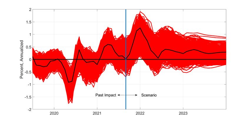
Figure 9 shows a much more muted response of headline PCE inflation to gasoline
price shocks in early 2020, with a trough of -6 percentage points compared to -9 percentage
points in Figure 3, and peaks of 4 percentage points each in early and late 2021, compared
with 5 and 6 percentage points, respectively, in Figure 3. This impression is confirmed in
Table 2, which shows an impact of only 1.8 percentage points in 2021, 0.4 percentage points
in 2022, and 0.1 percentage points in 2023. Clearly, users of headline PCE inflation would be
less concerned with the $100 oil scenario than users of the headline CPI inflation rate.
The results for the trimmed mean PCE inflation rate in Figure 10 also differ
substantially from those for core CPI inflation in Figure 4. Whereas the magnitude of the
decline in 2020 with 0.8 percentage points is similar, the maximum effect of 0.4 percentage
points in early 2021 and 0.7 percentage points at the end of 2021 is substantially smaller than
for core CPI inflation, even though we start at a higher base level in Figure 10. Nevertheless,
the impact on annual trimmed mean PCE inflation in 2022 and 2023 in Table 2 is broadly
similar to that for core CPI inflation. The main difference is that the effect on trimmed mean
inflation is somewhat smaller and less persistent. Additional analysis based on replacing the
trimmed mean inflation rate in model (2) by core PCE inflation indicates that the impact on
annual inflation in the core PCE (defined as the PCE excluding food and energy) would be
160.3 percentage points in 2021, 0.4 percentage points in 2022, and 0.1 percentage points in
2023.
5. Implications for Year-Over-Year Inflation Rates
Whereas our analysis has been based on monthly observations, much of the policy debate is
concerned with the evolution of year-over-year changes in the price level. This distinction is
important because measuring inflation as a trailing 12-month moving average may affect the
duration of the deflationary and inflationary effects of gasoline price shocks, their magnitude
and their timing.
As Figure 11 shows, by this metric, gasoline price shocks caused a sustained decline
in headline CPI inflation in 2020, which was overcome only in the second quarter of 2021.
Under the scenario, the peak effect of gasoline price shocks on headline CPI inflation is only
3 percentage points in late 2021 (compared with 5.7 percentage points in Figure 3 for the
monthly rate). However, the inflationary effects of the hypothesized gasoline price shocks by
construction decline much more slowly in 2022 than in Figure 1. Qualitatively similar results
hold for headline PCE inflation, except at a lower level. The peak effect of higher gasoline
prices under the scenario is reduced from 3.6 percentage points to 1.8 percentage points. By
comparison, the effect on year-over-year core CPI inflation, core PCE inflation and trimmed
mean PCE inflation at the end of 2022 reaches 0.4, 0.4 and 0.2 percentage points,
respectively, before gradually declining to zero in 2023, at which point they actually exceed
headline inflation.
6. Concluding Remarks
In this paper, we presented simple tools that allow researchers to understand the impact of
oil price fluctuations on inflation and inflation expectations, both based on historical data and
under hypothetical scenarios about the future evolution of the price of crude oil. The methods
discussed in this paper are of general interest to central bankers and macroeconomists.
17Recently, even more aggressive oil price scenarios have been advanced. For example, the
Bank of America is now predicting that the price of Brent crude oil will reach $120 a barrel
by June 2022, well above the scenario we considered. It would be straightforward to examine
the implications of such more extreme scenarios using the tools we employed in this paper.
While we have analyzed the impact of oil price scenarios from the point of view of the
United States, which simplifies the analysis because oil is traded in U.S. dollars, our analysis
could be easily extended to other countries with the important difference that the oil price
under a given scenario would have to be expressed in the domestic currency of those
countries first, before computing the implied path of gasoline price inflation.
References
Arias, J.E., Rubio-Ramirez, J.J., and D.F. Waggoner (2018), “Inference based on structural
vector autoregressions identified by sign and zero restrictions: Theory and
applications,” Econometrica, 86, 685-720. https://doi.org/10.3982/ECTA14468
Binder, C. (2018), “Inflation expectations and the price at the pump,” Journal of
Macroeconomics, 58, 1-18. https://doi.org/10.1016/j.jmacro.2018.08.006
Binder, C., and C. Makridis (2021), “Stuck in the seventies: Gas prices and macroeconomic
expectations,” Review of Economics and Statistics, forthcoming.
https://doi.org/10.1162/rest_a_00944
Blanchard, O.J. (1986), “The Wage Price Spiral,” Quarterly Journal of Economics, 101, 543-
565. https://doi.org/10.2307/1885696
Christiano, L., Eichenbaum, M., and C. Evans (1999), “Monetary Policy Shocks: What Have
We Learned and to What End?”, Handbook of Macroeconomics, eds. M. Woodford
and J. Taylor, North Holland. https://doi.org/10.1016/S1574-0048(99)01005-8
Clark, T.E., and S.J. Terry (2010), “Time variation in the inflation passthrough of energy
prices,” Journal of Money, Credit and Banking, 42, 1419-1433.
18https://doi.org/10.1111/j.1538-4616.2010.00347.x
Coibion, O., and Y. Gorodnichenko (2015), “Is the Phillips curve alive and well after all?
Inflation expectations and the missing disinflation,” American Economic Journal:
Macroeconomics, 7, 197-232. https://doi.org/10.1257/mac.20130306
Conflitti, C., and R. Cristadoro (2018), “Oil prices and inflation expectations”, Banca d’Italia
Occasional Papers No. 423.
Conflitti, C. and M. Luciani (2019). “Oil price pass-through into core inflation,” Energy
Journal, 40, 221-247. https://doi.org/10.5547/01956574.40.6.ccon
Dolmas, J., and E.F. Koenig (2019), “Two Measures of Core Inflation: A Comparison,”
Federal Reserve Bank of St Louis Review, 101, 245-258.
https://doi.org/10.20955/r.101.245-58
Inoue, A., and L. Kilian (2021), “Joint Bayesian inference about impulse responses in VAR
models,” Journal of Econometrics, forthcoming.
https://doi.org/10.1016/j.jeconom.2021.05.010
Karlsson, S. (2013), “Forecasting Bayesian vector autoregressions,” in: G. Elliott and A.
Timmermann (eds.), Handbook of Economic Forecasting, 2, Amsterdam:
North-Holland, 2013, 791-897. https://doi.org/10.1016/B978-0-444-62731-5.00015-4
Kilian, L. (2009), “Comment on ‘Causes and Consequences of the Oil Shock of 2007-08’ by
James D. Hamilton,” Brookings Papers on Economic Activity, 1, Spring, 267-278.
Kilian, L., and H. Lütkepohl (2017), Structural Vector Autoregressive Analysis, Cambridge
University Press: Cambridge. https://doi.org/10.1017/9781108164818
Kilian, L., and L.T. Lewis (2011), “Does the Fed Respond to Oil Price Shocks?,” Economic
Journal, 121, 1047-1072. https://doi.org/10.1111/j.1468-0297.2011.02437.x
Kilian, L., and C. Vega (2011), “Do energy prices respond to U.S. macroeconomic news? A
test of the hypothesis of predetermined energy prices,” Review of Economics and
19Statistics, 93, 660- 671. https://doi.org/10.1162/REST_a_00086
Kilian, L. and X. Zhou (2020), “Does Drawing Down the U.S. Strategic Petroleum Reserve
Help Stabilize Oil Prices?” Journal of Applied Econometrics, 35, 673-691.
https://doi.org/10.1002/jae.2798
Kilian, L. and X. Zhou (2021), “Oil prices, gasoline prices and inflation expectations,”
manuscript, Federal Reserve Bank of Dallas.
Lee, I. (2021), “Oil could surge above $100 in the event of a cold winter - and spark inflation
that drives the next macro crisis, BofA says,” Markets Insider, Oct 1, 2021.
Wong, B. (2015), “Do inflation expectations propagate the inflationary impact of real oil
price shocks? Evidence from the Michigan Survey,” Journal of Money, Credit and
Banking, 47, 1673-1689. https://doi.org/10.1111/jmcb.12288
20Figure 1: Indicators used in the VAR analysis, 1990.4-2021.9
NOTES: All data have been demeaned and expressed in percentage points.
Figure 2: Estimated responses to gasoline price shock in model (1), 1990.4-2021.9
NOTES: The core and headline inflation rates have been annualized. The set of impulse
responses shown in black is obtained by minimizing the absolute loss function in expectation
over the set of admissible structural models, as discussed in Inoue and Kilian (2021). The
responses in the corresponding 68% joint credible set are shown in a lighter shade.
21Figure 3: Monthly headline CPI inflation caused by gasoline price shocks, 2019.6-
2023.12
NOTES: Authors’ computations based on estimated model (1). The expected path is shown
as the black line. The other lines capture the uncertainty about this path based on an
approximation to the 68% joint credible set.
Figure 4: Monthly core CPI inflation caused by gasoline price shocks, 2019.6-2023.12
NOTES: See Figure 3.
22Figure 5: 1-Year household inflation expectation caused by gasoline price shocks,
2019.6-2023.12
NOTES: See Figure 3.
Figure 6: 5-Year household inflation expectation caused by gasoline price shocks,
2019.6-2023.12
NOTES: See Figure 3.
23Figure 7: The path of the WTI price of crude oil under the $100 oil scenario
Dollar/Barrel
100
80
60
40
20
0
Sep-21 Nov-21 Jan-22 Mar-22 May-22 Jul-22 Sep-22 Nov-22
NOTES: The September 2021 observation is included as a benchmark. Under the scenario,
the oil price remains at $80 until December 2023. The prices beyond December 2022 are not
included above to improve the readability of the plot.
Figure 8: Estimated responses to gasoline price shock in model (2), 1990.4-2021.9
NOTES: The trimmed mean and headline inflation rates have been annualized. The set of
impulse responses shown in black is obtained by minimizing the absolute loss function in
expectation over the set of admissible structural models, as discussed in Inoue and Kilian
(2021). The responses in the corresponding 68% joint credible set are shown in a lighter
shade.
24Figure 9: Monthly headline PCE inflation caused by gasoline price shocks, 2019.6-
2023.12
NOTES: Authors’ computations based on estimated model (2). The expected path is shown
as the black line. The other lines capture the uncertainty about this path based on an
approximation to the 68% joint credible set.
Figure 10: Monthly trimmed mean PCE inflation caused by gasoline price shocks,
2019.6-2023.12
NOTES: See Figure 9.
25Figure 11: Year-over-year inflationary effects of gasoline price shocks, 2019.6-2023.12
Percent
NOTES: Estimates based on models (1) and (2). All results shown are based on 12-month
trailing averages of the monthly Bayes estimates in Figures 3, 4, 9 and 10.
Table 1: The contribution of gasoline price shocks to the variability in inflation and
inflation expectations
Variables in model (1) Percent share of variance explained
Headline CPI Inflation 62.9
[59.5, 66.4]
CPI Inflation excluding Food and Energy 6.9
[4.1, 9.8]
1-Year Inflation Expectation 37.5
[30.7, 44.3]
5-Year Inflation Expectation 14.3
[7.6, 21.1]
NOTES: Authors’ computations based on model (1). 68% error bands in parentheses.
26Table 2: Inflationary effects by year under the $100 oil scenario (Percentage points)
2021 2022 2023
Annual Headline CPI Inflationa 2.99 0.40 -0.18
[2.42, 3.54] [0.14, 1.36] [-0.35, 0.30]
Annual CPI Inflation excluding 0.47 0.38 0.30
Food and Energya [0.17, 0.57] [0.14, 0.72] [0.02, 0.42]
1-Year Inflation Expectationa 0.56 0.76 0.23
[0.32, 0.62] [0.52, 1.04] [0.09, 0.54]
5-Year Inflation Expectationa 0.05 0.15 0.12
[-0.02, 0.09] [0.09, 0.24] [0.06, 0.22]
Annual Headline PCE Inflationb 1.78 0.44 0.12
[1.85, 2.46] [0.02, 0.81] [-0.26, 0.16]
Annual PCE excluding Food 0.43 0.33 0.09
and Energyc [0.25, 0.57] [0.07, 0.46] [-0.06, 0.18]
Annual Trimmed Mean PCE 0.33 0.37 0.07
Inflationb [0.17, 0.39] [0.25, 0.63] [0.02, 0.33]
a
Based on estimates of model (1). b Based on estimates of model (2). c Based on estimates
obtained when replacing the trimmed mean PCE inflation in model (2) by core PCE inflation.
NOTES: Authors’ computations based on estimates of models (1) and (2). The table shows
the average value of the estimated path of each variable over the 12 months of a given year.
The corresponding 68% error bands are shown in parentheses.
Table 3: The contribution of gasoline price shocks to the variability in inflation and
inflation expectations
Variables in model (2) Percent share of variance explained
Headline PCE Inflation 54.8
[51.2, 58.5]
Trimmed Mean PCE Inflation 14.6
[10.1, 19.0]
1-Year Inflation Expectation 37.0
[30.4, 43.7]
5-Year Inflation Expectation 14.3
[7.7, 21.0]
NOTES: Authors’ computations based on model (2). 68% error bands in parentheses.
27You can also read


