The infection fatality rate of COVID-19 in Stockholm - Technical report
←
→
Page content transcription
If your browser does not render page correctly, please read the page content below

The infection fatality rate
of COVID-19 in Stockholm
– Technical report
This title be downloaded from: www.folkhalsomyndigheten.se/publicerat-material/.

© Public Health Agency of Sweden, Year 2020.

Article number: 20094-2

                                                 3
Table of contents
Abstract ....................................................................................................................... 5
1. Introduction ............................................................................................................. 6
1.1 Background ........................................................................................................ 6
1.2 Summary of method and results ........................................................................... 8
2. Data ........................................................................................................................ 9
2.1 Data sources ...................................................................................................... 9
2.2 Variables .......................................................................................................... 10
2.3 Sample ............................................................................................................ 11
2.4 Descriptive statistics .......................................................................................... 11
3. Method .................................................................................................................. 14
3.1 Estimation of deaths ......................................................................................... 14
3.2 Estimation of the total number of infected ........................................................... 15
3.3 Inference for and interpretation of the IFR .......................................................... 16
4. Results .................................................................................................................. 17
4.1 Generalizability of the results ............................................................................. 18
4.2 Excess mortality................................................................................................ 19
5. Sensitivity analysis .................................................................................................. 21
5.1 Specification of the estimation sample ................................................................ 21
5.2 The PCR testing window .................................................................................... 22
6. Discussion .............................................................................................................. 24
References................................................................................................................. 25
A Figures .............................................................................................................. 26
B Tables ............................................................................................................... 28
C Death dynamics ................................................................................................. 29
4Abstract
We estimate the infection fatality rate of COVID-19 in the Stockholm region in
Sweden, for cases with symptom onset 21–30 March. We estimate the number of
deaths, i.e. the numerator, prospectively, using data from an individual-level
database of all confirmed cases in Sweden. The number of infections in the
denominator is based on an estimate of the total number of infections (including
unreported) per confirmed case. This estimate is based on a survey in which a
random sample of the population in the Stockholm region was tested for SARS-
CoV-2 by means of a Polymerase Chain Reaction test.
Our point estimate of the infection fatality rate is 0.6%, with a 95% confidence
interval of 0.4–1.1%. For the age group 0–69 years, we get an estimate of 0.1%
(c.i. 0.1–0.2%), and for those of age 70 years or older our estimate is 4.3% (c.i.
2.7–7.7%).
Most of the uncertainty in our estimations concerns the relationship between the
total number of infections and confirmed cases. We assess how the estimate of this
relationship, and thus the infection fatality rate, varies with alternative assumptions
about the time window during which an ongoing or previous infection can be
detected with Polymerase Chain Reaction testing. Additional analysis of excess
mortality in the Stockholm region during the period studied suggests that our
estimate is likely to be conservative.
51. Introduction
The aim of this study is to estimate the infection fatality rate (IFR) of COVID-19 in
the Stockholm region in Sweden, henceforth referred to simply as Stockholm. The
IFR, defined as the ratio of deaths to the total number of infected (including
unreported cases) is among the key parameters for evaluating the consequences of
the SARS-CoV-2 pandemic. Given a scenario for the number of infected persons,
the IFR provides an estimate of the number of expected deaths. The IFR can also
be of interest from a modelling perspective, as it can be used to estimate the
number of previous infections, from data on deaths. This method can provide more
accurate estimates of the total number of infected, given that confirmed deaths are
typically more accurately recorded than confirmed infections (relative to their
respective true totals).
1.1 Background
Stockholm has so far been the epicenter of the SARS-CoV-2 pandemic in Sweden.
Stockholm has 2,377,000 inhabitants, and thereby accounts for 23% of the Swedish
population. As of 25 May, Stockholm has 11,271 PCR-confirmed cases,
accounting for 33% of the cases in Sweden. 1 As of 25 May, there were 1,942
confirmed deaths reported in Stockholm, corresponding to a population fatality rate
of 0.1%, and accounting for 48% of all deaths in Sweden.
Many families from Stockholm travelled to the Alps for skiing when the schools
had their winter holiday week from 24 February to 1 March. This coincided with
the outbreak in the region Lombardy in northern Italy, which reported its first case
on 21 February and the first death on the 22th, indicating that the infection was
already widespread at that point. Many Swedes, and persons from Stockholm in
particular, were infected in Italy, Austria and to some extent in Iran, where an
outbreak started around the same period. Stockholm was thus seeded by many
returning travellers in the beginning of March, and the pandemic took off rather
quickly.
The trajectory of the epidemic for all confirmed cases in Stockholm is illustrated in
Figure 1, with the date of symptom onset on the horizontal axis and the number of
incident cases on the vertical axis (a similar graph for Sweden is shown in Figure
A.1 in Appendix A).
1 Health care workers have been tested to a larger extent outside of Stockholm. When these are
excluded, Stockholm accounts for 41% of the Swedish cases.
6Figure 1: Epidemic trajectory by case type in Stockholm
Figure 1 also highlights the Swedish testing policy, which so far can be divided
into three phases. The first phase lasted until 12 March and was characterized by
testing and tracing of imported cases and their contacts.
The second phase started 13 March, a few days after that the Public Health Agency
of Sweden declared that the spread of the infection was domestic and society-wide.
In this phase, the scope of testing was narrowed down to mostly include suspected
cases requiring hospital care, and to some extent health care workers.
The third phase maintains focus on symptomatic cases requiring care, but also to a
much larger extent includes proactive testing of care personnel in hospitals and
nursing homes, with mild or no symptoms. The third phase starts gradually from
the first half of April and overlaps with the second phase. As of writing, this third
phase is still ongoing. A transition to a fourth phase has begun, however,
characterized by broader testing, e.g. among those employed in jobs deemed to be
vital for the society.
71.2 Summary of method and results
We estimate the number of deaths, the IFR numerator, using detailed individual
case data from SmiNet, the Swedish reporting system and database for notifiable
diseases, which is matched to other sources of register data, including the official
death records. These data, which include all laboratory-confirmed COVID-19 cases
in Sweden, allow us to track deaths prospectively for all cases in our estimation
sample, defined to include those with symptom onset any time during 21–30 March
(indicated by the shaded area in Figure 1). We estimate the total number of
infections associated with these cases, i.e. those infected at the same point in time,
by multiplying the sample size of our estimation sample with an estimate of the
total number of infections (including unreported) per confirmed case. We infer the
relationship between total and reported cases from a compartmental
epidemiological model calibrated to the share of persons who tested positive for
SARS-CoV-2 in a Polymerase Chain Reaction (PCR) test included in Hälsorapport,
a survey administered in a random sample of the population in Stockholm between
26 March and 2 April. Our estimation framework accounts for uncertainty both in
the estimate of deaths and in the number of infected persons.
Our point estimate of the IFR is 0.6%, with a 95% confidence interval of 0.4–1.1%.
For the age group 0–69 years, the IFR is 0.1% (c.i. 0.1–0.2%), and for those of age
70 years or older we get an estimate of 4.3% (c.i. 2.7–7.7%). Comparisons between
the cases in our estimation sample and those in the rest of Stockholm and Sweden
suggest that our results are generalizable.
The number of deaths is precisely estimated and insensitive to how we specify the
estimation sample. Instead, most of the uncertainty in our estimations concerns the
number of infections per confirmed case. We assess how the estimate of this
relationship, and thus of the IFR, varies with alternative assumptions about the time
window during which an ongoing or previous infection can be detected with PCR
testing. Based on rather limited existing knowledge about non-hospitalized cases,
we assume a testing window of ten days.
Our estimation framework only includes deaths from confirmed cases, but
additional analysis of excess mortality in Stockholm suggests that our IFR estimate
is likely to be conservative.
82. Data
2.1 Data sources
We use two main data sources. For estimating deaths, we use SmiNet, the Swedish
reporting system and database for notifiable infectious diseases. SmiNet contains
all laboratory-confirmed (by PCR test) cases of COVID-19 in Sweden. The
database consists of individual-level records including date of symptom onset, test
and death, as well as demographic characteristics such as sex, age, region etc.
Moreover, the SmiNet data used in our analysis have been matched with the deaths
records maintained by the Swedish Tax Agency, medical risk factors from the
Swedish patient register and information about ICU care from the intensive care
register SIR.
For the estimation of the total number of infections, we calibrate an
epidemiological compartmental model both to SmiNet and to data from the
Stockholm sub-sample of the survey Hälsorapport (meaning “Health report” in
Swedish). Hälsorapport is a web-based longitudinal panel survey conducted by the
Public Health Agency of Sweden together with the national statistics office,
Statistics Sweden. It’s used to monitor ongoing or recent illness in the general
population, by asking respondents to report about what symptoms they had during
the past 24 hours and the past two weeks (e.g. fever, coughing, headache).
Recruitment to the survey is based on a stratified random sample of the Swedish
population aged 0–85. 2 During 26 April to 2 March, the Hälsorapport survey for
Stockholm was complemented with a self-administered PCR test intended to
estimate the population prevalence of COVID-19. The full results from and the
method of this survey are documented (in Swedish) in a previous report by Public
Health Agency of Sweden (2020b).
Briefly, 18 out 707 participants tested positive, corresponding to an estimate of
2.5% of the population in Stockholm, with a 95% confidence interval of 1.4–
4.1%. 3 The estimated prevalences across age groups were 2.8% for ages 0–15,
2.4% for ages 16–29, 2.6% for ages 30–59 and 2.0% for those of age 60+. None of
these differences were found to be statistically significant, although the statistical
power to detect such differences was small. We will thus maintain a null
hypothesis of an equal attack rate across age groups. We extend this assumption to
the population older than 85 years, even though we cannot assess it, given that this
age group was not included in the survey
2 For Stockholm, this implies that 98.3% of the population was covered by the sample frame.
3 Design weights and post-stratification weights accounting for non-response were applied in the
estimations.
92.2 Variables
Our main outcome variable is death attributable to COVID-19 among laboratory-
confirmed cases. Our data on deaths, and our definition of a COVID-19-
attributable death, correspond to the official statistics reported by the Public Health
Agency of Sweden, which are also reported to international institutions like the
European Center for Disease Control. A case is classified as a COVID-19 death if
1) reported as dead in SmiNet either directly by the treating doctor or by a
healthcare unit via the regional disease control unit; or 2) the case has died within
30 days from the test date, through matching the SmiNet database with official
deaths records (done routinely). 4 Note that deaths according to 1) may occur more
than 30 days after the test date, but in practice these account only for 0.9% of the
deaths in our estimation sample.
The number of laboratory-confirmed deaths is an underestimate of the total number
of deaths caused by COVID-19 (discussed in more detail in Section 4.2), but
provides a solid analysis framework, since every death is linked to a case record in
SmiNet and can thus be associated with date of symptom onset etc, as well as
individual characteristics.
We use various date variables from, or derived from, the SmiNet data. The
statistics date is the date when the case is reported in SmiNet. In median, the case
is reported 1 days after the test date, which is the date when the test was taken. The
symptom onset date is the date when the case first noted symptoms, as reported to
the doctor. Symptom onset date is recorded for the majority of individuals in the
early phase of the outbreak, but to a lesser extent later on. This is because the
obligation for doctors to write a clinical case report was abolished 26 March
(Public Health Agency of Sweden, 2020c), for non-hospitalized cases.
For cases without a recorded symptom onset date, we impute it as the test date
minus four days, the median time between onset of symptoms and test date,
estimated from all Swedish cases with non-missing values for both dates. For the
few cases without a recorded test date, we impute the symptom onset date as the
statistics date (available for all cases), minus five days, the median time between
onset of symptoms and statistics date.
Note that whenever we refer to the date of death, we refer to the actual death date,
rather than the date that the death was reported.
From the Swedish patient register, we have information about whether the
individual had any medical risk factors related to e.g. heart, lungs, cancer or
diabetes. We use these to characterize our sample, by counting whether an
4If there is no recorded test date, the date of diagnosis is used to determine whether the death occured
within 30 days. If the date of diagnosis is missing, the statistics date, available for all cases, is used.
10individual had at least one or two of these risk factors. From the intensive care
register we have an indicator variable for whether a case was ever admitted to ICU.
2.3 Sample
Our estimation sample is a subset of 1,667 cases from the SmiNet data tested in
Stockholm and with a date of symptom onset during the ten-day period between
21–30 March. This period roughly matches the period of (potential) symptom onset
of those who were PCR-tested in the Hälsorapport survey, between 26 March and 2
April. Specifically, we assume that the median time window for testing positive is
ten days, starting at the day of symptom onset (discussed further in Sections 3.2
and 5.2).
We choose a narrow estimation sample with symptom onset close in time to the
Hälsorapport survey, to avoid having to assume that the relationship between total
infections and confirmed cases estimated from that survey is constant over time.
For practical purposes, we also need to look at cases a sufficiently long way back
in time, in light of the time from onset to death and the delay in reporting
(discussed further in Appendix C). We show, though, that our results are
insensitive to the choice of estimation sample in Section 5.1.
A symptom onset date was recorded for 62% of the cases in our estimation sample.
Among the rest of the cases, 100% had a recorded test date, which we used to
impute the symptom onset date as described in Section 2.2.
The shaded area in Figure 1 indicates the dates of symptom onset of our estimation
sample. Our estimation sample coincides with the second testing phase, i.e. mainly
characterized by domestically infected cases in contact with the health care system.
2.4 Descriptive statistics
Descriptive statistics for our estimation sample are shown in the left panel of Table
1 (the three left-most columns). The first columns shows all cases, the second
column excludes imported cases and health care workers, and the third column
shows all cases that died.
The share of deaths among all cases, i.e. the case fatality rate (CFR), is 25.9%.
Men are slightly overrepresented among cases (54.2%), even more so among
deaths (57.4%). Living in a nursing home can be seen as a proxy for both old age
and underlying health problems. Among all cases in our estimation sample, 18.8%
are from nursing homes, but the share is twice as high (38.0%) among the deaths.
In terms of age profile, older persons are clearly overrepresented, e.g. those of age
70 or older account for 50.6% of the cases. The pattern is even more striking for
cases who died, as those of age 70 or older account for 85.9% of the deaths.
The share of cases in the estimation sample admitted to ICU at some point is 9.2%.
The corresponding figure for those who died was 10.2%. Excluding imported cases
11and health care workers doesn’t change the picture much from our full estimation
sample, since these cases only account for a small share of the total.
Table 1: Descriptive statistics
Estimation sample Stockholm Rest of Sweden
All No care Deaths All No care Deaths All No care Deaths
workers workers workers
Imported 0.8 0.0 2.6 0.2 3.4 0.8
case
Health care 4.6 0.2 16.8 0.2 39.0 0.1
worker
Male 54.2 55.2 57.4 46.8 51.6 54.0 38.2 49.6 56.1
Nursing 18.8 19.9 38.0 19.3 23.9 45.6 9.9 17.0 37.1
home
≥ 1 risk 69.9 71.7 91.6 65.2 72.8 92.0 50.2 67.5 91.5
factors
≥ 2 risk 49.7 51.9 76.8 45.7 53.4 76.8 30.2 46.1 73.8
factors
Intensive 9.2 9.2 10.2 6.7 7.8 9.2 5.3 8.3 11.0
care
Deceased 25.9 27.3 17.2 21.3 9.2 15.8
Age
0–29 4.4 4.1 0.0 6.8 5.7 0.2 12.6 7.3 0.2
30–49 16.9 15.3 1.2 21.3 15.7 1.2 28.5 17.9 1.2
50–59 15.3 14.8 5.8 16.6 12.9 3.7 18.6 13.9 2.4
60–69 15.5 15.3 7.2 12.7 13.1 7.4 11.9 12.3 6.9
70–79 17.8 18.7 25.5 14.4 17.7 22.8 9.8 16.4 21.4
80–89 20.7 21.8 38.9 17.8 22.0 39.6 12.2 20.9 42.5
90+ 9.5 10.0 21.5 10.4 12.8 25.2 6.4 11.1 25.3
Sample 1,667 1,579 432 11,271 9,091 1,942 22,572 13,110 2,087
size
The column ’No care workers’ excludes health care workers and imported cases. All variables are dichotomous and
presented as percentage shares.
In Figure 2, we show the distribution of death dates for our estimation sample (the
shaded area indicates the dates of symptom onset for the estimation sample). The
distribution has a rather long tail to the right, which highlights the importance of
studying cases sufficiently back in time, in order not to underestimate the number
of deaths. The onset-to-death delay and the reporting delay in death statistics is
looked at in more detail in Appendix C.
12Figure 2: Distribution of date of death in estimation sample
133. Method
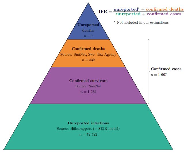
The IFR consists of two components that are estimated separately, the number of
deaths (the numerator) and the number of infections (the denominator). An
overview of these components and their data sources is shown in Figure 3.
Figure 3: The components and data sources of the IFR estimate
3.1 Estimation of deaths
We obtain our numerator by simply summing the number of deaths among the
cases in our estimation sample. It’s important to note, though, that deaths are
tracked prospectively, which is possible since we have individual-level data. We
thus avoid the bias which typically follows when using aggregated data, in which
case there will be a mismatch between the deaths in the numerator and the number
of associated infections in the denominator.
The number of deaths is a realization of a binomial random variable. We construct
a 95% confidence interval for the number of deaths by means of a parametric
bootstrap, drawing 1,000 replicates from a binomial distribution with parameters n
equal to the estimation sample size, and p equal to the CFR. The width of the lower
confidence interval is then computed as the distance between the median and the
2.5th percentile, and similarly with respect to the 97.5th percentile for the width of
the upper interval.
143.2 Estimation of the total number of infected
We compute the number of infected persons in our denominator by multiplying the
estimation sample size (1,667) with an estimate of the total number of infections
per confirmed case. We interpret this as the total number of incident cases that
were infected along with the cases in our estimation sample. 5
The relationship between total number of infections and confirmed cases is inferred
from a SEIR model, calibrated to the share of PCR-positives in the Hälsorapport
survey (see Section 2.1). This model has been used previously by Public Health
Agency of Sweden (2020a) to estimate the degree of underreporting and to forecast
the peak day of infected and the number of infected in Stockholm.
Essentially, the SEIR model fits an incidence of daily infections so as to match
both the trajectory of confirmed cases in SmiNet and the population prevalence of
PCR positives between 26 March and 2 April, as estimated from Hälsorapport. The
relationship between the fitted incidence and the incidence of confirmed cases is
what we’re interested in.
The assumed time window during which an ongoing or previous infection can be
detected with PCR testing is crucial for this calculation. Intuitively, a short testing
window implies high turnover in the stock of infected, and thus a large number of
infections, and vice versa. Public Health Agency of Sweden (2020a) used a time
window of five days, corresponding to the mean infectious period in the model
(1/γ), which yielded 78 infections per confirmed case. It’s, however, well-
established by now that the testing window is longer than the infectious period (see
e.g. Public Health Agency of Sweden, 2020d and additional references therein).
For this study, we thus use a more realistic length of ten days, which yields 44
infections per confirmed case. This is based in large part on Hu et al. (2020), who
report a median testing window of ten days. Their study is one of the few that
estimates the PCR testing window in a sample of mild and asymptomatic cases
recruited by means of contact tracing rather than among hospitalized patients.
Arguably, this corresponds better to the cases found in a population survey like
Hälsorapport. We assess the sensitivity of our results to the length of the testing
window and discuss the issue further in Section 5.2.
Besides this re-parametrization, the model has only been modified slightly, e.g. a
separate compartment for recovered individuals who still test positive has been
added. Since the model is already described in Public Health Agency of Sweden
(2020a), it will not be covered in more detail here.
Our estimator of the number of infections per confirmed case—and hence of the
total number of infections—is affected not only by the assumed PCR testing
5 We don’t know when the cases were infected, but this isn’t important for the validity of this
approach.
15window, but also by sampling variation in the estimator of the PCR prevalence. To
account for this, we use a parametric bootstrap approach, assuming that the PCR
prevalence estimator follows a beta distribution with shape parameters α = 14.56
and β = 553.92. 6 We draw 1,000 replicates from this distribution, whereafter we run
the model 1,000 times to get a bootstrap distribution for the number of infections
per confirmed case. We use this distribution to compute a confidence interval for
the total number of infections, using the same percentile-based method as for
deaths described in Section 3.1.
3.3 Inference for and interpretation of the IFR
We construct a bootstrap distribution for our IFR estimator by computing the IFR
from 1,000 deaths–infected pairs drawn from the respective bootstrap distributions
for deaths and infections (which are independent). Thereafter, we construct a 95%
confidence interval using the same percentile-based approach as for deaths and
infections, described in Section 3.1.
As mentioned in Section 2.1, we assume an equal attack rate across age groups.
The validity of our IFR estimator across all ages does not hinge on this assumption,
but it matters for the interpretation. In order to capture the difference in the fatality
rate across age groups, we also estimate age-conditional IFR’s for the age groups
0–69 and 70+, and for narrower age bands. In doing so, we multiply the number of
infected (the denominator) in each age group with the corresponding population
share in Stockholm, using the latest official population statistics pertaining to
December 2019, from Statistics Sweden. This method relies on the assumption of
an equal attack rate.
Arguably, an equal attack rate is a natural null hypothesis for the period studied
given that the infection circulated widely in the society. On the other hand, it’s
possible that those of age 70+ practiced social distancing to a larger extent, in line
with the official recommendations, or that they naturally have a lower contact rate.
If this is the case, we would underestimate the IFR for ages 70+, and overestimate
it for the 0–69 group.
6 The confidence interval around the prevalence 2.5% in Public Health Agency of Sweden (2020b)
was estimated using the Clopper-Pearson method, which uses beta distributions with different
parameters for the lower and the upper confidence interval limits, respectively. Our parametrization
represents the beta distribution which lies inbetween these distributions.
164. Results
The results for all ages are shown in the top panel of Table 2, with point estimates
on the first row and 95% confidence intervals in parentheses below. Based on the
1,667 cases in our estimation sample, we estimate the number of deaths quite
precisely to 432 (c.i. 397–464). Our estimate of the total number of infections is
74,089, corresponding to 44 infections per confirmed case. The wide confidence
interval 41,660–117,419 reflects considerable uncertainty in this estimate. Dividing
the number of deaths with the number of infections gives an IFR estimate of 0.58%
(c.i. 0.37–1.05%).
The bottom row panels of Table 2 show results conditional on age. Among 868
cases aged 0–69 years in our estimation sample, there are 61 deaths. We estimate
65,446 total infections in this group, corresponding to 75 infections per confirmed
case. This yields an IFR of 0.09%.
Table 2: IFR estimates for Stockholm
Population Cases Deaths Infected IFR (%)
share (%)
All ages 1,667 432 74,089 0.58
(397; 464) (41,660; 117,419) (0.37; 1.05)
Age 0–69 88.3 868 61 65,446 0.09
(47; 76) (36,800; 103,721) (0.06; 0.18)
Age 70+ 11.7 799 371 8,643 4.29
(344; 396) (4,860; 13,698) (2.67; 7.73)
In contrast, there are 371 deaths among 799 cases of age 70 years or older. With
an estimated 8,643 total infections in this group, there are 11 infections per
confirmed case, i.e. a much smaller share of unreported cases compared to the 0–69
age group. Since we have assumed a constant attack rate across age groups, this
simply reflects a higher probability of becoming a case for the 70+ age group, i.e.
an increased severity on average. Our estimate of the IFR for those aged 70 years
or above is 4.29%. This means that the risk of death given infection among the 70+
age group is 46 times higher than for the 0–69 age group.
More detailed age-conditional estimates are presented in Table B.1 in Appendix B.
From these results, it’s clear that there isn’t a jump in the IFR at age 70, but rather
a non-linear age gradient, which can be discerned both among those younger than
and those older than 70 years.
174.1 Generalizability of the results
We are interested in whether our IFR estimate is valid for the rest of Stockholm,
and for Sweden as a whole. We can assess this informally, by comparing the
characteristics of the estimation sample to all of the cases in Stockholm and to the
cases in the rest of Sweden. A simple comparison is misleading, however, since the
number of health care workers that have been tested has increased over time, and a
larger share of health care workers has been tested outside of Stockholm. Instead,
we focus our comparison of these samples after excluding health care workers and
imported cases, as shown in column 2 in respective column panel in Table 1. 7
Looking at demographics, there are more men in the estimation sample (55.2%)
than in Stockholm as a whole (51.6%) and than in the rest of Sweden (49.6%). This
could perhaps reflect underreporting of health care workers, who are
predominantly women. The age distribution is quite similar across samples, with
50.6% of age 70 or older in the estimation sample, 52.6% in Stockholm and 48.5%
in the rest of Sweden.
The share of cases from nursing homes in our estimation sample (19.9%) is lower
than in Stockholm (23.9%), but higher than in Sweden excluding Stockholm
(17.0%). The differences are not huge, but indicate that an overall IFR for
Stockholm, given the case distribution so far, would be somewhat higher than our
estimate of 0.6%, everything else equal. Analogously, the IFR would be somewhat
lower for Sweden. This pattern is similar when looking at risk factors. The share of
cases with at least one risk factor, e.g., are 71.7% for the estimation sample, 72.8%
for Stockholm and 67.5% for the rest of Sweden.
Overall, we believe that the differences in the sample characteristics are small
enough to generalize the results to both Stockholm as a whole and to the rest of
Sweden, with the caveat that the final IFR in each case will depend on the
particular distribution of cases in terms of age and underlying health. When
generalizing the results to Sweden as a whole, we might also want to consider that
Stockholm has a younger population than the rest of the country—in Stockholm,
the share of the population of age 70+ is 11.7%, whereas the corresponding figure
for Sweden is 14.8%. If we combine the age-conditional estimates for Stockholm
from Table 2 with the Swedish age distribution, we thus get a somewhat higher
IFR of 0.7%. This re-scaled number is based on the assumption that the attack rate
across ages is the same as in Stockholm, but this may or may not be true, e.g. if the
efforts to shield old people in general and in nursing homes in particular are more
successful than in Stockholm so far. 8
7Note that we cannot meaningfully compare the CFR across samples, due to right-censoring in
deaths.
8We also computed a nation-wide IFR by extrapolating on the estimated relationship between total
and confirmed cases from Stockholm, and using an estimation sample of cases from all of Sweden,
184.2 Excess mortality
Our IFR estimate is based on deaths of confirmed cases only. Yet, most countries,
including Sweden, have been reporting excess all-cause mortality not accounted for
by confirmed COVID-19 cases. An overview of all-cause mortality in Sweden
from 2016 is shown in Figure A.2 in Appendix A, from which it can be seen that
the level of excess mortality during the pandemic so far has been exceptionally
high, and clearly exceeding the mortality levels associated with past years’
seasonal influenza and the heat wave during the summer of 2018.
Figure 4: Weekly confirmed COVID-19 deaths and excess mortality in Stockholm
Figure 4 shows the weekly deaths of all confirmed cases in Stockholm during
weeks 12–19 (16 March to 10 May), grouped by our estimation sample and
remaining cases. The orange over-plotted line shows weekly excess mortality in
Stockholm during the same period, defined as the actual total number of deaths
except care workers (and imported cases), as these have been tested to larger extent outside of
Stockholm. This gives an IFR point estimate of 0.54%.
19minus a baseline estimated using the European Mortality Monitoring model
(MOMO). 9 We see that “unexplained” excess mortality—i.e. the part not accounted
for by confirmed COVID deaths—peaked in absolute terms during week 15, the
same week that confirmed deaths peaked, including deaths in our estimation
sample. Thereafter, the gap has closed gradually, presumably due to more
extensive testing. 10
During weeks 13–17, when 97% of the deaths in our estimation sample occurred,
the ratio of excess mortality to confirmed deaths in Stockholm was 1.24. When we
weight this ratio by the weekly shares of deaths in the estimation sample, we get a
factor of 1.28. Taken at face value, our IFR estimate should be adjusted upward
with the same factor. We can’t incorporate the excess mortality numbers formally
into our current estimation framework, however, since we cannot link the deaths to
any cases and hence not to any onset dates. In light of this, we’re therefore inclined
to view our original IFR estimates as conservative, rather than presenting adjusted
numbers. Future studies should analyze excess mortality more comprehensively,
perhaps combined with seroprevalence data, when available.
9 In short, the MOMO model fits a sinusoidal curve to deaths data from the past five years. Only
weeks during spring and autumn are used to fit the curve, since deaths during these weeks are less
likely to fluctuate from year-to-year due to seasonal influenza and extreme heat. For details, see
Gergonne et al. (2011).
10 During weeks 18–19, excess mortality was actually lower than confirmed deaths, indicating that
there would be fewer deaths than normal, if it wasn’t for the COVID deaths.
205. Sensitivity analysis
5.1 Specification of the estimation sample
We have chosen a narrow estimation sample close in time to the Hälsorapport
survey, to avoid having to assume that the relationship between the total number of
infections and confirmed cases estimated from that survey is constant over time. If
the relationship would indeed be constant—at least before the third test phase
including more health care workers—as assumed in Public Health Agency of
Sweden (2020a), then we could in principle define our estimation sample as we
like, given that we look sufficiently back in time to account for the time from onset
to death and the delay in reporting. This raises the question of whether the results
are robust to the specific date interval chosen for inclusion in the estimation
sample.
Figure 5: IFR as a function of date interval of estimation sample
As an extreme, we extended our original ten-day sample period by one week before
and one week after, giving us a 24-day sample including cases with symptom onset
21from 14 March to 6 April. 11 This sample includes 3,819 cases, of which 992 have
died, i.e. a CFR of 26.0%. This is very close to the CFR of 25.9% of our original
estimation sample. Since the scaling factor is constant, the IFR of the extended
sample thus becomes 0.58%, practically the same as for the narrow sample. 12
Next, we compute the IFR for all possible estimation samples within the period 14
March to 6 April, i.e. 300 samples of length 1 to 24 days. The results, which are
shown in Figure 5, are extremely robust to which dates are used. The mean of these
estimates is 0.58%, the mean weighted by the number of days used in the
estimation sample is 0.58%, and the 25th, 50th and 75th quantiles are 0.57%,
0.59% and 0.60%, respectively.
5.2 The PCR testing window
Figure 6 shows how the IFR point estimate would vary with different assumptions
of the PCR testing window, used for mapping the Hälsorapport survey estimate of
2.5% positive to an estimate of the total number of incident cases infected
alongside the cases in our estimation sample. Specifically, the shown range of 5–15
days implies a range of IFR’s from 0.3% to 0.7%, so the PCR testing window is
clearly an important parameter for our results.
We surveyed the literature of the PCR testing window (also known as the duration
of viral shedding) in order to come up with a valid parametrization for our
purposes. Our chosen value of ten days is based largely on Hu et al. (2020), as
already motivated in Section 3.2. This is, to the best of our knowledge, the only
study of the PCR testing window among contact-traced cases that weren’t recruited
in a hospital setting. For this reason, and even though it’s a single study of only 24
cases, we believe it’s more representative of infections picked up in a population
survey like Hälsorapport. However, we recognize that it would be valuable to have
more knowledge about the PCR testing window in non-hospitalized cases.
11 Including cases earlier back in time would put us in the first phase of the epidemic, characterized
mostly by imported cases, and going further ahead in time would lead to right-censoring in deaths.
12 Interestingly, the 95% confidence interval of 0.37–1.03% is not tighter than the interval for the
narrow sample, despite a larger sample size. This highlights that most of the variation comes from the
denominator.
22Figure 6: IFR estimate as a function of the PCR testing window
We also considered the following studies that included and presented results
separately for patients with milder infections. Zheng et al. (2020) report a median
testing window of 14 days in a subset of 22 hospitalized patients with mild disease
in China, which is shorter compared to the median of 21 days reported for 74
patients with severe disease. Yongchen et al. (2020) find a median testing window
of 10 days among 11 nonsevere hospitalized patients in China, and a median of 18
days among 5 asymptomatic cases. Other studies surveyed included both a mix of
mild, moderate and severe hospitalized cases, but did not report results by group.
There is considerable variation in the estimates, but such studies typically reported
median values of 12–20 days.
All of the studies considered were PCR tests based on sputum/saliva,
nasopharyngeal swabs or throat swabs, or some combination thereof, and were thus
judged to be relevant with respect to the test used in the Hälsorapport survey, in
which all of these methods were combined (Public Health Agency of Sweden,
2020b).
236. Discussion
We’ve estimated the IFR of COVID-19 to 0.6%, for persons in Stockholm with
symptom onset around the end of March, based on deaths of confirmed cases. We
find a clear age-gradient in the IFR, with persons of age 70 years or older having a
46-fold risk of dying compared to those younger than 70 years, according to our
estimates. Moreover, a sizeable share of the deaths can be attributed to cases from
nursing homes—38.0% of the deaths in our estimation sample and 41.2% of the
total number of deaths in Sweden as of 25 May.
Our results are similar to a handful of existing published results up to this point.
Russell et al. (2020) estimate an IFR of 0.6% for China (95% c.i. 0.2–1.3%), based
on re-scaling age-conditional IFR estimates from the Diamond Princess Cruise
Ship to the age-distribution of Chinese cases. Verity et al. (2020) estimate an IFR
of 0.7% for China (95% c.i. 0.4–1.3%). They assume an equal attack rate across
ages, and their estimate of the total share of infected is based on the share of PCR-
confirmed cases among international residents repatriated from Wuhan. Salje et al.
(2020) incorporate estimates from the Diamond Princess Cruise Ship in a
modelling framework and estimate an IFR of 0.7% for France (95% c.i. 0.4–1.0%).
There is substantial uncertainty in our estimations, due to the uncertainty in the
total number of infections. Yet, we believe that our estimates are more likely than
not to be conservative, due to the fact that we don’t account for unreported
COVID-19 deaths. Moreover, we argue that the results plausibly generalize to the
rest of Stockholm and to Sweden as a whole, but this should be assessed more
carefully in future studies. If seroprevalence data from a random population sample
becomes available in the future, this should help reducing the uncertainty about the
total number of infections.
24References
Gergonne, B., A. Mazick, J. O’Donnell, A. Oza, B. Cox, F. Wuillaume, et al. (2011). A European
algorithm for a common monitoring of mortality across Europe. Work package 7 report. Technical
report, Copenhagen: Statens Serum Institut. https://euromomo.eu/.
Hu, Z., C. Song, C. Xu, G. Jin, Y. Chen, X. Xu, H. Ma, W. Chen, Y. Lin, Y. Zheng, et al. (2020).
Clinical characteristics of 24 asymptomatic infections with COVID-19 screened among close contacts
in Nanjing, China. Science China Life Sciences, 1–6.
Public Health Agency of Sweden (2020a). Estimates of the peak-day and the number of infected
individuals during the COVID-19 outbreak in the Stockholm region, Sweden February – April 2020.
Technical report, Public Health Agency of Sweden.
https://www.folkhalsomyndigheten.se/publicerat-material/publikationsarkiv/e/estimatesof-the-peak-
day-and-the-number-of-infected-individuals-during-the-COVID-19-outbreak-in-thestockholm-region-
sweden-february–april-2020/.
Public Health Agency of Sweden (2020b). Förekomsten av COVID-19 i region Stockholm, 26 mars–3
april 2020. Technical report, Public Health Agency of Sweden.
https://www.folkhalsomyndigheten.se/publicerat-material/publikationsarkiv/f/forekomstenav-
COVID-19-i-region-stockholm-26-mars3-april-2020/.
Public Health Agency of Sweden (2020c). Ändring i föreskrifter (HSLF-FS 2015:7) om anmälan av
anmälningspliktig sjukdom i vissa fall. Technical report, Public Health Agency of Sweden.
https://www.folkhalsomyndigheten.se/publicerat-material/publikationsarkiv/h/hslf-fs202010/.
Public Health Agency of Sweden (2020d). Vägledning om kriterier för bedömning av smittfrihet vid
COVID-19. Technical report, Public Health Agency of Sweden.
https://www.folkhalsomyndigheten.se/publicerat-material/publikationsarkiv/v/vagledningom-
kriterier-for-bedomning-av-smittfrihet-vid-COVID-19/.
Russell, T. W., J. Hellewell, C. I. Jarvis, K. Van Zandvoort, S. Abbott, R. Ratnayake, S. Flasche, R.
M. Eggo, W. J. Edmunds, A. J. Kucharski, et al. (2020). Estimating the infection and case fatality
ratio for coronavirus disease (COVID-19) using age-adjusted data from the outbreak on the
diamond princess cruise ship, february 2020. Eurosurveillance 25(12), 2000256.
Salje, H., C. T. Kiem, N. Lefrancq, N. Courtejoie, P. Bosetti, J. Paireau, A. Andronico, N. Hoze, J.
Richet, C.-L. Dubost, et al. (2020). Estimating the burden of sars-cov-2 in France. Science.
Verity, R., L. C. Okell, I. Dorigatti, P. Winskill, C. Whittaker, N. Imai, G. Cuomo-Dannenburg, H.
Thompson, P. G. Walker, H. Fu, et al. (2020). Estimates of the severity of coronavirus disease
2019: a model-based analysis. The Lancet infectious diseases.
Yongchen, Z., H. Shen, X. Wang, X. Shi, Y. Li, J. Yan, Y. Chen, and B. Gu (2020). Different
longitudinal patterns of nucleic acid and serology testing results based on disease severity of
COVID-19 patients. Emerging Microbes & Infections (just-accepted), 1–14.
Zheng, S., J. Fan, F. Yu, B. Feng, B. Lou, Q. Zou, G. Xie, S. Lin, R. Wang, X. Yang, et al. (2020).
Viral load dynamics and disease severity in patients infected with SARS-CoV-2 in Zhejiang province,
China, January-March 2020: retrospective cohort study. British Medical Journal 369.
25A Figures
Figure A.1: Epidemic trajectory by case type in Sweden
26Figure A.2: Weekly deaths and MOMO baseline (95% c.i.) in Sweden from week 1, 2016,
to week 19, 2020
27B Tables
Table B.1: IFR estimates for Stockholm by age
Population Cases Deaths Infected IFR (%)
share (%)
Age 0–49 66.6 355 5 49,324 0.01
(1; 9) (27,735; 78,170) (0.00; 0.02)
Age 50–59 12.5 255 25 9,277 0.27
(16; 34) (5,216; 14,702) (0.15; 0.50)
Age 60–69 9.2 258 31 6,845 0.45
(20; 41) (3,849; 10,848) (0.25; 0.88)
Age 70–79 7.7 296 110 5,737 1.92
(93; 127) (3,226; 9,091) (1.16; 3.40)
Age 80–89 3.1 345 168 2,333 7.20
(151; 186) (1,312; 3,697) (4.54; 12.84)
Age 90+ 0.8 158 93 574 16.21
(81; 105) (323; 909) (10.11; 29.50)
28C Death dynamics
When estimating the IFR, one needs to properly account for the dynamics between
infection (or symptom onset) and death. Conceptually, we should think of whether
a case dies or not as a Bernoulli random variable. Conditional on death, the timing
of death is also random, with a range from the day of symptom onset up to over
one month later. Moreover, we need to account for reporting delay in the death
statistics. The majority of deaths in Sweden are reported within ten days from the
actual death date, but with a tail of cases that lag up to another 1–2 weeks. This
implies that we should only consider cases with symptom onset at least 40–50 days
in the past. Even so, we may miss some deaths that occur late and are reported late,
but we could disregard these cases for practical purposes. This study uses data up
to 25 May 2020, which means that we can study cases up to the first week of April,
if we want to avoid right-censoring.
Figure C.3 shows the distribution of days from symptom onset to death, for all
cases in Sweden. The mode is 10 days, the mean is 12, and the 25th, 50th and 75th
percentiles are 7, 10 and 15, respectively.
Figure C.3: Distribution of time from symptom onset to death among all Swedish cases
29To see the importance of both the time from onset to death and the delay in
reporting, for computing fatality rates, consider Figure C.4, in which the CFR is
plotted by date of symptom onset up until today (the shaded area indicates the dates
of symptom onset for the estimation sample). Sweden and Stockholm are shown
separately, and imported cases and health care workers have been excluded for
better comparability across samples and over time. We see that the CFR peaks in
the beginning of April, but after around a week into April, it starts to fall steeply,
due to the combined effects of time from onset to death and delay in reporting. For
this reason, we shouldn’t compare CFR’s across samples with different shares of
recent cases, e.g. between our estimation sample and the Stockholm sample.
Figure C.4: Case fatality rate by date of symptom onset in Stockholm and Sweden
(excluding imported cases and health care workers)
From Figure C.4, we also note that the CFR in Stockholm has been somewhat
higher than in Sweden as a whole, but the gap appears to close over time. The grey
shaded area indicates the date range of our estimation sample
30______________________________
The Public Health Agency of Sweden is an expert authority with responsibility for public health
issues at a national level. The Agency develops and supports activities to promote health, prevent
illness and improve preparedness for health threats. Our vision statement: a public health that
strengthens the positive development of society.
Solna Nobels väg 18, SE-171 82 Solna. Östersund Campusvägen 20. Box 505, SE-831 26 Östersund.
www.folkhalsomyndigheten.seYou can also read