The Mean Squared Prediction Error Paradox
←
→
Page content transcription
If your browser does not render page correctly, please read the page content below

Munich Personal RePEc Archive

The Mean Squared Prediction Error
Paradox

Pincheira, Pablo and Hardy, Nicolas

Universidad Adolfo Ibáñez, Universidad Finis Terrae

24 April 2021

Online at https://mpra.ub.uni-muenchen.de/107403/
MPRA Paper No. 107403, posted 30 Apr 2021 07:17 UTC

The Mean Squared Prediction Error Paradox1

         Pablo Pincheira Brown♣                               Nicolás Hardy§

              School of Business                       School of Economics and Business

         Universidad Adolfo Ibáñez                         Universidad Finis Terrae

                                           April 2021

                                            Abstract

In this paper, we show that traditional comparisons of Mean Squared Prediction Error
(MSPE) between two competing forecasts may be highly controversial. This is so because
when some specific conditions of efficiency are not met, the forecast displaying the lowest
MSPE will also display the lowest correlation with the target variable. Given that
violations of efficiency are usual in the forecasting literature, this opposite behavior in
terms of accuracy and correlation with the target variable may be a fairly common
empirical finding that we label here as "the MSPE Paradox." We characterize "Paradox
zones" in terms of differences in correlation with the target variable and conduct some
simple simulations to show that these zones may be non-empty sets. Finally, we illustrate
the relevance of the Paradox with two empirical applications.

JEL Codes: C52, C53, G17, E270, E370, F370, L740, O180, R310

Keywords: Mean Squared Prediction Error, Correlation, Forecasting, Time Series, Random Walk.

1
    Corresponding Author: Pablo Pincheira-Brown: Diagonal Las Torres 2640, Peñalolén, Santiago,
Chile. Email: pablo.pincheira@uai.cl.
♣
    We are thankful to Universidad Adolfo Ibáñez for financial support through the Concurso de
Investigación Individual 2020. We are also thankful to Juan Pablo Medina, Rodrigo Wagner and
participants of the seminars of the Business School, Universidad Adolfo Ibáñez, for very
constructive comments.

                                                1
1. Introduction
"How wonderful that we have met with a paradox. Now we have some hope of making progress."
Niels Bohr.

In this paper, we show that traditional comparisons of Mean Squared Prediction Error
(MSPE) between two competing forecasts may be highly controversial. This is so because
when some specific conditions of efficiency are not met, the forecast displaying the lowest
MSPE will also display the lowest correlation with the target variable. Given that
violations of efficiency are usual in the forecasting literature, this opposite behavior in
terms of accuracy and correlation with the target variable may be a fairly common
empirical finding that we label here as the MSPE paradox2.

It is safe to say that MSPE is one of the most popular measures in the forecast evaluation
literature, with a long tradition in both empirical and theoretical works. Just as an
anecdotal illustration of its relevance, the acronym "MSPE" is mentioned 77 times in West's
(2006) survey. The rationale for using MSPE as a loss function is as follows: MSPE is a
statistical measure of accuracy, then, a forecast displaying a low MSPE is an accurate
forecast that, on average, will be close to the target variable. Some of the most iconic
empirical contributions in economic forecasting (such as those of Meese and Rogoff (1983,
1988), Goyal and Welch (2008), Stock and Watson (2003), and Timmermann (2008)) rely
partially or completely on MSPE comparisons. Due to its importance and tractability, it is
not surprising that many theoretical works in this literature treat MSPE as a leading case
(e.g., Diebold and Mariano (1995), West (1996), Giacommini and White (2006)).

An alternative avenue to evaluate predictive ability could consider the association
between the forecast and the target variable: the tighter the association is, the better the
forecast is. Probably the simplest association measure between two random variables, X
and Y, is the correlation between them. According to this intuition, a forecast more closely
related to Y would be superior to another forecast not as closely related to Y. In other
words, a forecast with a higher correlation with Y should be preferable to another forecast
displaying a lower correlation.

Interestingly, in this paper, we show analytically and empirically that the forecast with the
lowest MSPE does not necessarily display the highest correlation (what we call the MSPE
Paradox). We show that both approaches are equivalent when forecasts meet some

2
 Violations of efficiency in the forecast literature are found across multiple variables in a number of articles.
See for instance, Ince and Molodtsova (2017); Joutz and Stekler (2000); Ang, Bekaert and Wei (2007); Bentancor
and Pincheira (2010); Patton and Timmermann (2012); Nordhaus (1987); Pincheira and Álvarez (2009);
Pincheira and Fernández (2011) and Pincheira (2012, 2010) just to mention a few.

                                                       2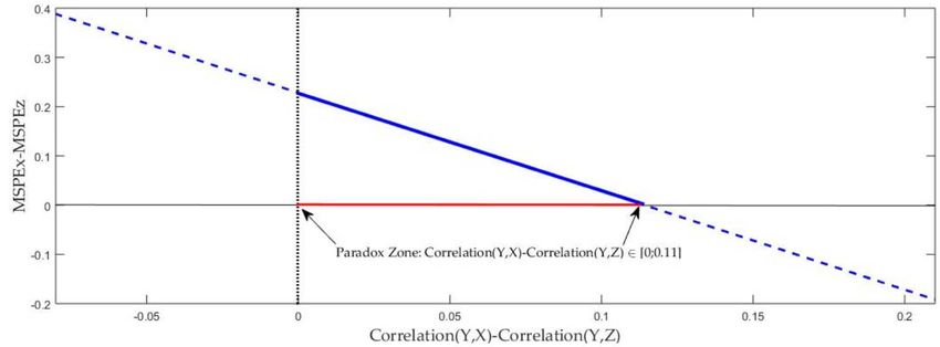
conditions of efficiency (Mincer and Zarnowitz (1969)). Given that violations of efficiency
are usual in the forecasting literature (see footnote 2), this opposite behavior in terms of
accuracy and correlation with the target variable may be a fairly common empirical
finding.

We offer a characterization of “Paradox zones” in terms of the differences in correlation
with the target variable. Moreover, we carry out simple simulations to show that these
Paradox zones are, in general, non-empty sets. As a matter of fact, our analysis shows that
we could have an extreme case in which a totally uncorrelated forecast with the target
variable could be superior in terms of MSPE to an alternative forecast displaying a positive
correlation with the same target variable. Our empirical illustration supports this idea.

Finally, we show the relevance of the MSPE Paradox with two empirical applications in
which some of the most accurate forecasts are, in fact, the worst in terms of correlations
with the target variable. Both illustrations are related to the commodity-currencies
literature. In the first exercise, we predict the returns of eleven commodities with the
exchange rates of five commonly studied commodity-exporting economies. In the second
exercise, we evaluate several exchange rates forecasts of the same five commodity-
exporting economies. In this case, we compare the predictions of the FX4cast survey with
some forecasts constructed with commodity returns and some usual benchmarks as well.

The rest of this paper is organized as follows. In section 2 we show with simple examples
what we call the MSPE Paradox. We warn the reader that in subsection 2.1 we will be
making very restrictive assumptions for the sake of clarity. Nevertheless, in subsection 2.2
we relax these assumptions to analyze the Paradox with more generality. In Section 3 we
offer a characterization of “Paradox zones”. In section 4 we illustrate the Paradox with
simple simulations whereas in section 5 we present two empirical illustrations. Finally,
section 6 concludes.

   2.      The MSPE Paradox

2.1 Simple examples

In this section we illustrate with simple examples what we call "The MSPE Paradox." We
use this name to label the fact that when comparing two competing forecasts for the same
target variable, it might be the case that the forecast displaying the lowest MSPE will also
display the lowest correlation with the target variable.

                                              3
Let us consider { } to be a mean zero target variable with variance equal 1. At time , we
have two competing forecasts {              } and {        } for { }. It is important to notice that both
{    } and {     } are forecasts constructed with information previous to time t and that
they are taken as primitives (hence, we are not concerned here about parameter
uncertainty). For clarity of exposition, we drop the sub-indexes t in what follows. Let us
assume that the vector ( ,           , )′ is weakly stationary (so here we assume the existence of
second moments).

Example 1:

For example 1 we will also assume that both forecasts have the same non-negligible
variance: Var(X)=Var(Z)>0, that X is a mean zero forecast and that                           (    ) > 0. Many of
these assumptions are very restrictive, but they are useful to illustrate the Paradox.

Consider now the MSPE of both forecasts:

                                        = ( − ) ;                        = ( − )

and let us also define the corresponding Mean Squared Forecasts (MSF) as follows:

                                             = (      );             = (        )

Suppose now that we are interested in a traditional comparison of MSPE, then:

                    ∆            ≡           −             =    ( − ) − ( − )

                                 =(         −      ) − 2(            −      )

                         =(            −         ) − 2{     !( , ) −            !( , )}

        =(          −        ) − 2"#$%( ) &         %%( , )"#$%( ) −                   %%( , )"#$%( )'

                    =(           −         ) − 2"#$%( ){         %%( , ) −             %%( , )}

               =(        −            ) − 2"          −(       ) {       %%( , ) −        %%( , ) }

                =(           −          ) − 2"        {     %%( , ) −               %%( , ) } (1)

Eq.(1) illustrates an important result: the difference in MSPE depends not only on the
correlation between the forecasts with the target variable, but also on MSF that are not
directly linked to properties of the target variable. The problem in this illustration relies on
a "magnitude" effect associated to the term (                   −          ): A high MSF of a forecast could
more than offset its high correlation with the target variable and therefore the forecast
itself could be outperformed by another less informational forecast with a lower MSF. In

                                                       4
other words, in this example, traditional MSPE comparisons give a natural advantage to
"small forecasts”, that is to say, forecasts with small MSF.

Example 2:

As a second example, let us consider a different econometric context, but similarly
simplistic, in which Z is a zero-forecast. Consequently, #$%( ) =                      !( , ) =    = 0.
Furthermore, let us also assume that             = 0, Var(X) > 0 and that Var(Y) = 1. We will have
then

                     ∆      ≡                −            =       ( − ) − ( − )

                              =(         −        ) − 2(          −     )

                         =(         −        ) − 2{       !( , ) −      !( , )}

                                        =(       ) − 2{       !( , )}

                         =(         ) − 2"#$%( )"#$%( ){                %%( , )}

                                =            − 2"             {   %%( , )}

then if "        >2      %%( , ) > 0 we will have that                             >       despite that
  !( , ) >      !( , ) = 0. This is, of course, an extreme situation. The use of MSPE in
this case, will suggest that the forecast with no association whatsoever with the target
variable is preferable to another forecast with a tighter association. The problem in this
example is that MSPE comparisons would fail to detect the usefulness of forecast X if its
magnitude (       ) overshadows its informational content.

2.2 A general case

Let us now leave behind our simplifying assumptions to show a more general picture of
the MSPE Paradox. We will analyze two leading cases: a case in which Y, X and Z have all
positive variances and a case in which Y and X have positive variances but Z is just a
constant c that might or might not be equal to zero. Beyond weak stationarity, we will also
assume that Corr(Y,X)
A4) Corr(Y,X)

nesting model introduces noise into its forecasts through the estimation of parameters
that, under the null, are equal to zero. This effect inflates the sample MSPE of the model
with additional parameters. Our decomposition resembles the findings by Clark and West,
and to some extent, it is even more general. Both Clark and West and us similarly argue
that a plain look at MSPE comparisons may be misleading in some circumstances, given
that they can be affected by several distortions. In the case of Clark and West, those
distortions arise from parameter estimation error. In our approach, these distortions arise
at the population level by comparing apple and oranges: forecasts with very different
magnitude effects or very different biases. In other words, even at the population level, we
may observe that some forecasts have a natural advantage in terms of MSPE relative to
others, despite of being far less informational relative to its competitors.

      3. Some simple theoretical results

In the following we will assume, without loss of generality, that                           %%( , ) ≥         %%( , ) if
Z has positive variance. In case that Z has zero variance, we will assume, without loss of
generality, that           !( , ) ≥       !( , ) = 0. In this setup the Paradox will exist whenever
         −                > 0. As we are considering the two leading cases of positive and zero
variance for Z, we will denote by Ω the variance-covariance matrix of the (Y,X,Z)’ vector
and by Ω the variance-covariance matrix of the (Y,X)’ vector.

Proposition 1: Let Z be a constant-forecast (say,                    = 0 ∀ ). Let us also assume that

                                             2345 6 7         :9(:     6)
                                                         −                  >0
                                             "8(9)8( )       "8(9)8( )

                                                                     2345 6 7        :9(:   6)
Then we will find the Paradox iif             %%( , ) ∈ [0;                      −               ).
                                                                     "8(9)8( )       "8(9)8( )

Corollary 1: If in Proposition 1 we set                = 0 = 0, we will find the Paradox iif                  %%( , ) ∈
       2345             :9:
[0;               −               ). Moreover, in the particular case in which                        = 0, we will find
      "8(9)8( )       "8(9)8( )
                                          "8( )
the Paradox iif           %%( , ) ∈ [0;           ).
                                          "8(9)

Proof of Proposition 1.

Notice that in this case we have ( ) = 0,                      = 0 and #( ) =               !( , ) = 0.

Here eq.(3.2) could also be written as

                      ∆           =       − 0 − 2&        %%( , )"#( )#( ) +                 (        − 0)'

                                                          7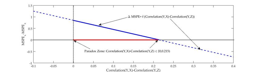
As     !( , ) = 0, we will have the Paradox whenever                             %%( , ) ≥ 0 and ∆                              > 0.
Imposing this last condition we get

       ∆           > 0⇔          − 0 − 2&         %%( , )"#( )#( ) +                    (       − 0)' > 0 (4)

                                                        −0               (        − 0)
                                 %%( , ) <                         −
                                                 2"#( )#( )            "#( )#( )

                                                                        2345 6 7            :9(:       6)
Therefore we will have the Paradox iif             %%( , ) ∈ [0;                        −                   )∎
                                                                        "8(9)8( )           "8(9)8( )

The proof of Corollary 1 follows simply by setting c=0.

Proposition 2 next shows an equivalent result for the case in which Z is a forecast with
positive variance.

Proposition 2: Let Z be a forecast with positive variance. Let Δ =                               %%( , ) −                    %%( , )
and suppose that

                      −                %%( , ) B"#( ) − "#( )C                      (       −          )
                                 −                                           −                             >0
                  2"#( )#( )                      "#( )                           "#( )#( )

Then we will find the Paradox iif

                                2345 234D        EFGG(9, )B"8( ) "8( )C           :9(:      : )
                      Δ ∈ [0;                −                                −                   ).
                                 "8(9)8( )                 "8( )                  "8(9)8( )

Proof of Proposition 2.

Reorganizing eq.(3.1) we get

 ∆           =       −          −2&     %%( , )"#( )#( ) −                   %%( , )"#( )#( ) +                           (      −       )'

=          −        − 2"#( )         %%( , ) B"#( ) − "#( )C − 2"#( )"#( )Δ − 2                                       (        −     ) (5)

We will find the Paradox whenever ∆                   > 0 and Δ ≥ 0, which is equivalent to

                             −               %%( , ) B"#( ) − "#( )C                             (         −      )
               0≤Δ<                     −                                               −
                         2"#( )#( )                        "#( )                            "#( )#( )

                                                                        2345 234D               EFGG(9, )B"8( ) "8( )C
And the Paradox condition is simply given by Δ ∈ [0;                                        −                                        −
                                                                         "8(9)8( )                             "8( )
:9(:   : )
             )∎
"8(9)8( )

                                                       8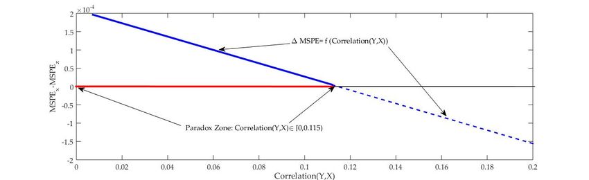
It is also interesting to explore if the Paradox is a simple consequence of the traditional
variance-bias trade-off so widely explored in the forecasting literature. It is well known
that a biased forecast could be superior to an unbiased forecast in terms of MSPE, if the
bias in the first forecast is associated to an important decrease in the variance of the
forecast error. To explore this possibility, we analyze the Paradox when comparing two
equally biased forecasts, so that the potential presence of the Paradox in this scenario
cannot be attributed to a variance-bias trade-off. The following corollary to proposition 2
addresses this case:

Corollary 2: If in Proposition 2 we set         =       , then we will find the Paradox iif

                                    8( ) 8( )       EFGG(9, )B"8( ) "8( )C
                          Δ ∈ [0;               −                            ).
                                    "8(9)8( )                "8( )

Notice that if V(X) = V(Z) then the Paradox is impossible as the Paradox zone is the empty
set. Put differently, our decomposition becomes

                              −             = −2"#( )#( ){           %%( , ) −         %%( , )}

which implies that differences in MSPE are equivalent to differences in correlations.

Nevertheless, whenever #( ) ≠ #( ) the Paradox will be possible as long as

                       [#( ) − #( )N            %%( , ) B"#( ) − "#( )C
                                        −                                         >0
                        2"#( )#( )                         "#( )

For this condition to hold true we require either

                                       "#( ) + "#( )
                          %%( , ) <                           OP #( ) > #( )
                                            2"#( )

Or

                                       "#( ) + "#( )
                          %%( , ) >                           OP #( ) < #( )
                                            2"#( )

                                                    9
In subsection 4.2 we show some simple simulations showing a non-empty Paradox zone
when forecasts are equally biased and #( ) > #( ). Similarly, in the appendix we show
simulations for equally biased forecasts when #( ) < #( ) with the same conclusion: a
non-empty Paradox zone. In summary, the MSPE Paradox is not a direct consequence of
the traditional variance-bias trade-off as Corollary 2 and our simulations show that the
Paradox also emerges in the context of equally biased forecasts.
Next we will see that for the Paradox to exist we require inefficient forecasts. We need
some notation first: Let QR and QS be the forecast errors of X and Z, respectively. In other
words
uU ≡ −
uV ≡ −
Let us recall that X and Z are efficient forecasts à la Mincer and Zarnowitz (1969) as long as
!( , W* ) = !( , W+ ) = 0
(W* ) = (W+ ) = 0
Proposition 3: If X and Z are both efficient à la Mincer and Zarnowitz, then the Paradox is
impossible.
Proof of Proposition 3.
Notice that Y= X+uU = Z+uV , therefore
#( ) = #( ) + #(W* ) + 2 !( , W* )
#( ) = #( ) + #(W ) + 2 !( , W )
Under efficiency à la Mincer and Zarnowitz (1969) these expressions reduce to:
#( ) = #( ) +
#( ) = #( ) +
Where = ( − ) ; = ( − ) .
Therefore
∆ ≡ − = #( ) − #( )
10Notice also that under efficiency à la Mincer and Zarnowitz (1969) we will have that
!( , ) = !(X + uU , ) = #( ) > 0
!( , ) = !(Z + uV , ) = #( ) ≥ 0
Which means that
∆MSPE ≡ − = V(Z) − V(X)= Cov(Y, Z) − Cov(Y, X) (6)
If Z is just a constant c (case C1) then Cov(Y, Z) = V(Z) = 0. Therefore
∆MSPE ≡ − = −Cov(Y, X) < 0
And clearly !( , ) > %%( , ) = 0, so the Paradox is impossible.
If Z has positive variance (case C2) then Cov(Y, Z) = V(Z) > 0. Let us recall that, without
loss of generality, we are assuming that %%( , ) ≥ %%( , ) whenever Z has positive
variance. But
!( + W* , ) #( ) + !( , W* )
%%( , ) = =
"#( )#( ) "#( )#( )
"8( )
Then, under efficiency à la Mincer and Zarnowitz (1969) %%( , ) = .
"8(9)
"8( )
Following the same argument, %%( , ) = .
"8(9)
With these results, the assumption %%( , ) ≥ %%( , ) is equivalent to
"#( ) ≥ "#( )
This and eq.(6) implies that
∆MSPE ≡ − ≤0
so the Paradox is, again, impossible ∎
4. Simulations
In proposition 1 the existence of the Paradox relies on the following assumption:
2345 6 7 :9(: 6)
− >0
"8(9)8( ) "8(9)8( )
11Whereas in proposition 2 it relies on the following more complex assumption:
− %%( , ) B"#( ) − "#( )C ( − )
− − >0
2"#( )#( ) "#( ) "#( )#( )
To illustrate that these assumptions may hold true and that the “Paradox zone” may be a
non-empty set, we carry out a set of simple simulations. In each simulation, we show that
the Paradox zone coincides with the intervals derived in Section 3. Here we show three
different cases: i) Z as a zero-forecast with arbitrary parameters, ii) Z is a more general case
with arbitrary parameters, and iii) Z is a zero-forecast in the context of a data generating
process calibrated with exchange rates forecasts. In addition, in the appendix we consider
a case in which both forecasts display equal bias and V(Z) > V(X).
4.1 Simulation with a "zero-forecast."
Let us suppose that we want to compare two competing forecasts, X and Z, where Var(X) >
0 and Z is a "zero-forecast." According to corollary 1 in Section 3, the Paradox zone is
defined by
` ( ) ( )
%%( , ) ∈ [0; − )
2"#( )#( ) "#( )#( )
234* :(9):( )
To show that [0; − ) may be a non-empty region, we consider the
"8(9)8( ) "8(9)8( )
following simulation: We start by setting = 0.1, = 1, ( ) = 2 and ( ) = 2, then
from expression (4) we have
Δ = MSPEU − + = 1.8 − 2.8213 ∗ %%( , )
Keeping , , ( ) and ( ) constant, our decomposition is just a linear function
between Δ and Corr(X,Y), with a slope of -2.8213 and an intercept of 1.8. In order to
analyze this linear function without changing the slope nor the intercept, we generate
different values of %%( , ) just by changing EYX but keeping in mind that the
covariance matrix Ω must be positive definite:
( )−( ) − 1 − 0.1
Ω =c d=B C
− ( )−( ) − 0.1 1.99
We parameterize EYX = 0.1 + δ, where δ is a sequence of small positive incremental
changes of 0.001. Notice that the slope and the intercept of our linear function remain
unaltered in this simulation. In this case, the Paradox zone is given by %%( , ) ∈
7i
:h :(9):( )
g0; − g = [0; 0.638). In other words, despite that forecast Z has no
"8(9)8( ) "8(9)8( )
12covariance with Y, it outperforms the forecast X in terms of MSPE whenever %%( , ) ∈
[0; 0.638).
Figure 1: Illustration of the Paradox zone when Z is a zero-forecast.
Source: Author's elaboration
4.2 Simulation with a general forecast Z
We consider a more general case now in which #( ) ≠ 0. According to Proposition 2, the
Paradox zone is given by
2345 234D EFGG(9, )B"8( ) "8( )C :9(: : )
Δ≡ %%( , ) − %%( , ) ∈ [0; − − ).
"8(9)8( ) "8( ) "8(9)8( )
In order to show that this interval may be a non-empty region, we carry out the following
simulation: We start by setting = 1, = 0.7, = 1.1, = 0.6, = 1, ( ) = 3,
( ) = 1.5 and ( ) = 2.5. This implies the following values:
#( ) = 2.64; "#( ) = 1.6248; #( ) =1.5; "#( ) = 1.2247; #( ) = 0.5; "#( ) = 0.7071;
Corr(Y,Z)=0.0870 and ( − ) = 0.
Then using expression (5) we have
Δ = MSPEU − + = 0.8536 − 3.9799 ∗ Δ
Keeping , , , , , ( ), ( ) and ( ) constant, our decomposition is just a
linear function between Δ and Δ with an approximate slope of -3.98 and an
approximate intercept of 0.85. In order to draw this linear function without affecting its
slope and intercept, we generate different values of Δ just by changing EYX but keeping in
mind that the following covariance matrix Ω must be positive definite:
3 − 0.6 − 0.6 ∗ 1 0.7 − 0.6 ∗ 1
Ω =l − 0.6 ∗ 1 2.5 − 1 1.1 − 1 ∗ 1 m
0.7 − 0.6 ∗ 1 1.1 − 1 ∗ 1 1.5 − 1
13We consider EYX = 0.15 + δ, where δ is a sequence of small positive increments of 0.001.
Notice that the slope and the intercept of our linear function remain unaltered in this
simulation. In this case, the Paradox zone is given by %%( , ) − %%( , ) ∈ [0; 0.215).
Figure 2: Illustration of the Paradox zone in a general framework.
Source: Author's elaboration
4.3 Simulation calibrated to exchange rates.
Here we show results when we compare a generic forecast X against a zero-forecast Z. So,
again, we are in the framework of Subsection 4.1. Differing from our first simulation in
which we consider arbitrary population parameters for our forecasts, here we pick our
parameters so to match sample moments of forecasts and exchange rates at the monthly
frequency. We use data of the Australian dollar obtained from Thomson Reuters
Datastream (our target variable Y). Our forecast X is simply a survey-based expectation for
the Australian exchange rate: we use data on professional exchange rate forecasts from
FX4Casts (previously known as The Financial Times Currency Forecaster and Currency
Forecasters’ Digest). Our database goes from October 2001 through May 2019.
Let us define our target variable as follows:
= ln( p ) − ln( p q)
Where p is the Australian Dollar (spot) at time t, and is simply the three-month
cumulative log-return. Let
= ln( q) − ln( p q)
where q is the FX4CASTS three-month ahead forecast for the Australian Dollar (e.g.,
the forecast for p , and is simply the forecast of the three-month ahead cumulative
return. We set the parameters of our simulations using the following sample moments:
= 0.0045, = −0.0010, ( ) = 0.0042 and ( ) = 0.0002
14This implies the following values (rounding to the fourth decimal):
#( ) = 0.0042; "#( ) = 0.0647; #( ) =0.0002; "#( ) = 0.0141; = −0.00005.
Then from expression (4), we have
Δ = MSPEU − + = 0.0002 − 0.0018 ∗ %%( , )
Keeping , , ( ) and ( ) constant, our decomposition is just a linear function
between Δ and Corr(X,Y), with a slope of -0.0018 and an intercept of 0.0002 (both
values rounded at the fourth decimal). In order to analyze this linear function without
changing the slope nor the intercept, we generate different values of %%( , ) just by
changing EYX but keeping in mind that the following covariance matrix Ω must be
positive definite:
( )−( ) −
Ω =c d
− ( )−( )
We consider EYX = 0 + δ, where δ is a sequence of small positive increments of 0.00001.
Notice that the slope and the intercept of our linear function remain unaltered in this
:h 7 i
simulation. In this case, the Paradox zone is given by %%( , ) ∈ g0; −
"8(9)8( )
:(9):( )
g = [0; 115). In other words, despite that forecast Z has no covariance with Y, it
"8(9)8( )
outperforms the forecast X in terms of MSPE whenever %%( , ) ∈ [0; 115).
Figure 3: Paradox zone with parameters calibrated to exchange rates
Source: Author's elaboration
155. Empirical illustrations of the MSPE Paradox
In this section we illustrate the Paradox with two empirical applications using
commodities and commodity currencies. In both cases, we will assume for simplicity that
population moments are well approximated by their sample counterparts.
5.1 The Paradox in commodity forecasts
Our first empirical illustration is inspired by the commodity-currencies literature. Chen,
Rogoff and Rossi (2010, 2011) seminal papers report strong predictive ability from the
exchange rates of some exporting countries such as Australia, Canada, Chile, New
Zealand and South Africa to some country-specific commodity indices. Additionally,
Pincheira and Hardy (2019, 2021) find strong predictive ability from the same currencies to
some base-metal prices.
In this context, we construct and compare different forecasts for 11 series of commodities
(aluminum, copper, lead, nickel, zinc, tin, LMEX, gold, silver, S&P GSCI, and platinum)
using the exchange rates of Australia, Canada, Chile, New Zealand and South Africa
(relative to the U.S dollar)3. The econometric specifications for our forecasts closely follow
Pincheira and Hardy (2019, 2021):
Δ = rΔ R t + εt ( 1)
Where Δ stands for the log-difference of a commodity price, Δ p is the log-difference
of a generic exchange rate, r is a regressor coefficient and εt is the error term. Note that we
are only evaluating one-step-ahead forecasts. The database is collected from Thomson
Reuters Datastream, considering monthly closing prices on commodity prices and
exchange rates (relative to the U.S dollar). In this analysis, we consider exclusively a
period in which all the economies pursue a pure flotation exchange rate regime; hence our
database goes from October 1999 through May 2019 (a total of T=236 observations for each
series).
In addition to the five forecasts generated by each exchange rate using (M1), we also
consider the forecast of a Driftless Random Walk (a zero-forecast, DRW), a Random Walk
(a forecast with the historical mean, RW), and an AR(1). Finally, the parameter r in (M1),
and the parameters of the AR(1) and the RW are estimated by OLS and updated with
rolling windows of R=48 monthly observations. Notice that all our forecasts are evaluated
out-of-sample, with a total of P=T-R=188 predictions.
3 The S&P GSCI was formerly known as the Goldman Sachs Commodity Index.
16Table 1: Evaluation of commodity forecasts with correlations with the target variable
and RMSPE.
(1) (2) (3) (4) (5) (6) (7) (8) (9)
Australia Canada Chile NewZealand SouthAfrica AR(1) RW DRW
S&P GSCI
Correlation 0.070 -0.023 0.147 -0.118 0.031 0.151 -0.065 -
RMSPE 0.067 0.067 0.066 0.069 0.067 0.066 0.067 0.066
LMEX
Correlation 0.049 -0.025 0.146 -0.178 -0.046 0.161 0.009 -
RMSPE 0.068 0.067 0.067 0.069 0.068 0.067 0.067 0.066
Aluminum
Correlation 0.029 -0.068 0.139 0.007 -0.087 0.137 -0.043 -
RMSPE 0.063 0.063 0.062 0.063 0.063 0.063 0.063 0.062
Notes: RMSPE stands for Root MSPE. Source: Author's elaboration
Table 1 reports our results when predicting GSCI, LMEX and aluminum4. First, 12 out of
21 non-zero forecasts have a positive correlation with the target variable, suggesting some
useful information in those forecasts. Notably, the DRW is the forecast with the lowest
RMSPE in the three commodities, despite having zero covariance with the target variable.
Second, note that the forecasts for each commodity show very similar RMSPE, but very
different correlations. For instance, the RMSPE for the LMEX goes between 0.066 and
0.069, but the correlations vary between -0.178 and 0.161. In other words, relative to the
maximums we find changes of around 4% in RMSPE and changes of around 210% in
correlations.
Third, there are some cases of paradoxes worth to be mentioned. For instance, for the
LMEX, the forecast of the AR(1) has a particularly high correlation of 0.161; nevertheless,
the DRW has a lower RMSPE. Moreover, the forecast constructed with the Australian
dollar has a correlation of 0.049, but notably, it has greater RMSPE than the forecast
constructed with the Canadian dollar, even though the latter has a negative correlation of -
0.025.
Figures 4 and 5 display the differences in MSPE and correlations between two forecasts
using rolling windows of 48 observations. Figure 4 compares two different forecasts for
aluminum: one constructed with the Australian Dollar and the other with the South
African Rand. Figure 5 reports our results when forecasting the LMEX with the Australian
4 Results for the rest of commodities are presented in Table A1 in the Appendix. With subtleties, some entries
of Table A1 also illustrate the Paradox. For instance, in the case of Zinc, the RMSPE ranges from 0.087 to 0.090.
Notably, with this commodity, the forecast constructed with the Chilean peso is the only one with a positive
correlation with the target variable, and at the same time, it exhibits a RMSPE of 0.090. In other words, the
forecast with the Chilean peso is the best in term of correlations, and one of the worsts in terms of RMSPE.
17and the Canadian Dollar. In both figures, whenever the differences in MSPE and
correlations have the same sign, we have the MSPE Paradox. Notably, both figures suggest
that the Paradox may appear quite often.
Figure 4: Differences in MSPE and Correlations using rolling windows. Forecasting
aluminum returns with the Australian and South African exchange rates.
Notes: Figure 4 displays the differences in MSPE and correlations between two competing forecasts, using
rolling windows of 48 observations. In this illustration the target variable is aluminum one-month returns. We
compare a forecast using the Australian Dollar with another using the South African Rand. Whenever both
series have the same sign, we have the MSPE Paradox. The differences in MSPE have been scaled so the left
axis represents both differences in MSPE and differences in correlations. Source: Author's elaboration
18Figure 5: Differences in MSPE and Correlations using rolling windows. Forecasting
LMEX with the Australian and Canadian exchange rates.
Notes: Figure 5 displays the differences in MSPE and correlations between two competing forecasts using
rolling windows of 48 observations. In this illustration the target variable is LMEX one-month returns. We
compare a forecast using the Australian Dollar with another using the Canadian Dollar. Whenever both series
have the same sign, we have the MSPE Paradox. The differences in MSPE have been scaled so the left axis
represents both differences in MSPE and differences in correlations. Source: Author's elaboration
5.2 The Paradox in exchange rates forecasts
In our second empirical illustration, we evaluate the predictive relationship between
commodities and commodity-currencies, but in the opposite direction (i.e., the ability of
fundamentals to predict exchange rates). Previous studies like Chen et al. (2010), Engel
and West (2005), and Ferraro et al. (2015) have evaluated this predictive performance with
rather weak results. For instance, Ferraro et al. (2015) conclude that the ability of
commodity prices to predict exchange rates is unstable and appears only for some
commodities at some frequencies. Chen et al. (2010) find evidence that exchange rates can
predict commodity prices at the quarterly frequency; nevertheless, there is little evidence
in the opposite direction. Moreover, Engel and West (2005) conclude that there is very
weak evidence of Granger-causality from fundamentals to exchange rates, yet results in
the opposite direction are more encouraging.
Due to the evidence reported in Ferraro et al. (2015), Chen et al. (2010) and Pincheira and
Hardy (2019, 2021) we consider the following commodities as predictors for exchange
rates: Aluminum, LMEX, Oil and a commodity index (MSCI GSCI). The commodity-
19currencies considered here are the same than in Chen et al. (2010): Australia, Canada,
Chile, New Zealand and South Africa.
In addition to our forecasts constructed with commodities, we evaluate the predictive
performance of the exchange rates FX4cast survey considered in previous studies such as
Ince and Molodtsova (2017)5. The main sources for our data are Datastream (for the case of
commodities) and FX4cast (for the exchange rates and their respective forecasts). Due to
data availability in FX4cast, we consider the following sample periods at the monthly
frequency: Australia (August 1986 through May 2019), Canada (August 1986 through May
2019), Chile (October 2001 through May 2019), New Zealand (December 1993 through May
2019) and South Africa (October 2001 through May 2019).
Our econometric specifications are very simple, mainly inspired by Pincheira and Hardy
(2019, 2021):
{
Δ R tvw = x yΔ zv +} v~
z|
Where Δ p v~ stands for the log-difference of a generic exchange rate at time t+h.
Δ zv stands for the log-difference of a generic commodity price. The number of lags
"p" is determined with AIC in each case, using the first 48 monthly observations. We
update estimates of the parameters for our forecasts using rolling windows of R=48
observations. Additionally, as in Subsection 5.1, we consider forecasts from a RW (a
forecast using the historical mean), a DRW (a zero-forecast) and an AR(p) (where "p" in
each case is determined again using AIC with the first 48 observations). We report out-of-
sample results for h=3 and h=6. Consequently, for h=3 we report results of the 3-months
ahead FX4cast survey and, for h=6, we report the 6-months ahead FX4cast survey6. Finally,
y is a regressor coefficient and } v~ is an error term.
5FX4cast considers five different horizons: 1, 3, 6, 12 and 24-months ahead. Nevertheless, the 1-month and the
24 months-ahead surveys are only available since May 2008 for all the exchange rates; for this reason, we only
use in this exercise the 3-, 6- and 12-months ahead forecasts.
6 One-step-ahead results (i.e., h=1) are available upon request.
20Table 2: Evaluation of exchange rate forecasts with correlations with the target variable
and RMSPE.
Australia h=6
(1) (2) (3) (4) (5) (6) (7)
FX4cast 6 Rolling AR(p) LMEX GSCI Oil WTI
Correlation 0.083 -0.051 -0.036 0.000 -0.039 -0.016
RMSPE 0.043 0.033 0.033 0.033 0.034 0.034
Canada h=6
Correlation 0.166 0.008 0.077 -0.076 -0.093 -0.088
RMSPE 0.026 0.023 0.022 0.024 0.024 0.024
Chile h=6
Correlation 0.088 -0.060 -0.027 -0.068 -0.062 -0.035
RMSPE 0.036 0.034 0.033 0.035 0.036 0.036
NewZealand h=6
Correlation 0.069 -0.053 -0.028 0.000 -0.049 0.048
RMSPE 0.047 0.038 0.038 0.038 0.038 0.037
SouthAfrica h=6
Correlation -0.004 -0.043 -0.052 0.007 0.083 0.056
RMSPE 0.052 0.046 0.048 0.048 0.047 0.047
Notes: RMSPE stands for Root MSPE, h is the forecasting horizon and FX4cast 6 is the 6 months-ahead forecast.
“Rolling” simply represents the forecast using the historical mean. Source: Author's elaboration
Table 2 shows some striking results7. First of all, with one exception (the South African
Rand), FX4CAST is always the forecast displaying the highest correlation with the target
variable, and notably, at the same time, it is always the forecast displaying the worst
RMSPE. For instance, for the Australian Dollar, FX4CAST has a RMSPE about 30% higher
than the other forecasts, despite the fact that it is the only forecast with a positive correlation
with the target variable.
Second, in three out of our five exchange rates, the forecast displaying the lowest RMSPE
has also a zero or negative correlation with the target variable; in other words, the “most
accurate” forecast is frequently one of the worsts in terms of correlations. Notably, in Table
2 we do not find any cases in which the forecast displaying the highest correlation exhibits
simultaneously the smallest RMSPE.
7 Results for h=3 are presented in Table A2 in the Appendix. With subtleties, some entries of Table A2 also
illustrate the Paradox. For instance, for the case of South Africa, every forecast displays a RMSPE of 0.048. This
result suggests that the six forecasts are similarly accurate. However, the correlation of the forecasts with the
South African rand ranges from -0.099 to 0.087; in other words, relative to the maximum, we observe
differences of more than 213%.
21All in all, Tables 1 and 2 support the main message of our paper: Sometimes, a set of
competing forecasts may exhibit a similar RMSPE (i.e., they are “similarly accurate”), and,
at the same time, they may have important differences in terms of correlations with the
target variable. In this scenario, no one would be surprised if no differences whatsoever
were found between our competing forecasts using traditional tests of equality in MSPE
(e.g., Diebold and Mariano (1995) and West (1996)), despite the fact that our forecasts
contains fairly different information about the future evolution of the target variable.
6. Concluding remarks
In this paper we show that traditional comparisons of Mean Squared Prediction Error
(MSPE) between two competing forecasts may be highly controversial. This is so because
when some specific conditions of efficiency are not met, the forecast displaying the lowest
MSPE will also display the lowest correlation with the target variable. Given that violations
of efficiency are usual in the forecasting literature, this opposite behavior in terms of
accuracy and correlation with the target variable may be a fairly common empirical finding
that we label here as "the MSPE Paradox."
We characterize "Paradox zones" in terms of differences in correlation with the target
variable and conduct some simple simulations to show that these zones may be non-empty
sets. Moreover, our analysis shows that we could have an extreme case in which a forecast
and a target variable are independent random variables, which speaks of a useless forecast,
yet, in terms of MSPE, this useless forecast might outperform a useful forecast displaying a
positive correlation with the target variable.
Finally, we illustrate the relevance of the MSPE Paradox with two empirical applications in
which some of the most accurate forecasts in terms of MSPE are, in fact, some of the worst
in terms of correlations with the target variable.
Our paper emphasizes the need to look beyond MSPE when evaluating two or more
competing forecasts, as a blind search for the minimum out-of-sample MSPE forecast may
lead to an incorrect evaluation of the information contained within those predictions. In
light of these results, an interesting avenue for future research is the elaboration of a simple
asymptotically normal test to evaluate two competing forecasts according to their
correlations with the target variable.
227. References
1. Ang, A., G. Bekaert and M. Wei. (2007) Do macro variables, asset markets, or
surveys forecast inflation better? Journal of Monetary Economics, Volume 54, issue 4,
1163-1212.
2. Bentancor, A. and P. Pincheira. (2010) Predicción de errores de proyección de
inflación en Chile. El Trimestre Económico, Vol (0) 305, 129-154. (In Spanish).
3. Chen, Y.-C., Rogoff, K. S., and Rossi, B. (2010). Can Exchange Rates Forecast
Commodity Prices ? Quarterly Journal of Economics, 125(August), 1145–1194.
4. Chen, Y.-C., Rogoff, K. S., and Rossi, B. (2011). Predicting Agri-Commodity Prices:
An Asset Pricing Approach, World Uncertainty and the Volatility of Commodity
Markets, ed. B. Munier, IOS.
5. Clark, T. E., and West, K. D. (2006). Using out-of-sample mean squared prediction
errors to test the martingale difference hypothesis. Journal of Econometrics, 135(1-2),
155-186.
6. Clark, T. E., and West, K. D. (2007). Approximately normal tests for equal
predictive accuracy in nested models. Journal of Econometrics, 138(1), 291-311.
7. Diebold, F. X., and Mariano, Roberto, S. (1995). Comparing Predictive Accuracy.
Journal of Business and Economic Statics, 13(3), 253–263.
8. Engel C. and K. D. West (2005). Exchange Rates and Fundamentals. Journal of
Political Economy, June 2005, 113 (3), 485—517.
9. Ferraro, D., Rogoff, K., and Rossi, B. (2015). Can oil prices forecast exchange rates?
An empirical analysis of the relationship between commodity prices and exchange
rates. Journal of International Money and Finance, 54, 116-141.
10. Giacomini, R., and White, H. (2006). Tests of conditional predictive
ability. Econometrica, 74(6), 1545-1578.
11. Ince, O., and Molodtsova, T. (2017). Rationality and forecasting accuracy of
exchange rate expectations: Evidence from survey-based forecasts. Journal of
International Financial Markets, Institutions and Money, 47, 131-151.
12. Joutz, F. and H.O. Stekler (2000). An Evaluation of the Prediction of the Federal
Reserve. International Journal of Forecasting. 16: 17–38.
13. Meese, R, and Rogoff, K. (1983). Empirical exchange rate models of the seventies:
Do they fit out of sample? Journal of International Economics, 14, 3–24.
14. Meese, R., and Rogoff, K. (1988). Was it real? The exchange rate-interest differential
relation over the modern floating-rate period. The Journal of Finance, 43(4), 933-948.
2315. Mehra, Y.P. (2002). Survey measures of expected inflation: Revisiting the issues of
predictive content and rationality. Federal Reserve Bank of Richmond Economic
Quarterly 88, 17-36.
16. Mincer, J. A., and Zarnowitz, V. (1969). The evaluation of economic forecasts.
In Economic forecasts and expectations: Analysis of forecasting behavior and
performance (pp. 3-46). NBER.
17. Nordhaus, W. (1987). Forecasting efficiency: concepts and applications. The Review
of Economics and Statistics, Vol LXIX, N°4. November 1987.
18. Patton, A. and A. Timmermann (2012). Forecast Rationality Tests Based on Multi-
Horizon Bounds“. Journal of Business and Economic Statistics 30(1): 1–17.
19. Pincheira, P., and Hardy, N. (2019). Forecasting base metal prices with the Chilean
exchange rate. Resources Policy, 62(February), 256–281.
20. Pincheira, P., and Hardy, N. (2021). Forecasting Aluminum Prices with Commodity
Currencies. Resources Policy, forthcoming.
21. Pincheira, P. and N. Fernández. (2011). Corrección de algunos errores sistemáticos
de predicción de inflación. Monetaria, CEMLA, vol. 0(1), 37-61. (In Spanish).
22. Pincheira, P. (2010). A Real time evaluation of the Central Bank of Chile GDP
growth forecasts. Money Affairs, CEMLA, vol. 0(1), 37-73.
23. Pincheira, P. and R. Álvarez. (2009). Evaluation of short run inflation forecasts and
forecasters in Chile," Money Affairs, CEMLA, vol. 0(2), 159-180.
24. P. Pincheira. (2012). A joint test of superior predictive ability for Chilean inflation
forecasts. Journal Economía Chilena (The Chilean Economy), Central Bank of Chile,
vol. 15(3), 04-39, (In Spanish).
25. Souleles N. (2004). Expectations, heterogeneous forecast errors and consumption:
Micro evidence from the Michigan consumer sentiment surveys. Journal of Money,
Credit and Banking. 36, 39-72.
26. Stock, J. H., and Watson, M. (2003). Forecasting output and inflation: The role of
asset prices. Journal of Economic Literature, 41(3), 788-829.
27. Thomas, L.B., 1999. Survey measures of expected U.S. inflation. Journal of Economic
Perspectives, 13, 125-144.
28. Timmermann, A. (2008). Elusive return predictability. International Journal of
Forecasting, 24(1), 1-18.
29. Welch, I., and A. Goyal (2008). A comprehensive look at the empirical performance
of equity premium prediction. The Review of Financial Studies, 21(4), 1455-1508.
30. West, K. D. (1996). Asymptotic Inference about Predictive Ability. Econometrica,
64(5), 1067.
31. West, K. D. (2006). Chapter 3 Forecast Evaluation. Handbook of Economic
Forecasting, 1(05), 99–134.
248. Appendix
A.1 Forecasting commodities with commodity-currencies.
(1) (2) (3) (4) (5) (6) (7) (8) (9)
Australia Canada Chile NewZealand SouthAfrica AR(1) RW DRW
Copper
Correlation 0.008 -0.001 0.137 -0.267 -0.082 0.192 0.002 -
RMSPE 0.083 0.081 0.081 0.085 0.082 0.081 0.082 0.081
Gold
Correlation -0.112 -0.075 -0.171 0.027 -0.169 0.046 0.061 -
RMSPE 0.052 0.051 0.052 0.051 0.052 0.051 0.050 0.051
Lead
Correlation 0.148 0.062 0.138 0.129 0.051 0.075 0.048 -
RMSPE 0.094 0.095 0.094 0.094 0.095 0.095 0.094 0.094
Nickel
Correlation 0.030 -0.056 0.012 -0.116 -0.015 0.045 0.031 -
RMSPE 0.103 0.104 0.104 0.105 0.103 0.103 0.101 0.101
Tin
Correlation 0.037 -0.068 0.034 -0.074 -0.005 0.109 0.120 -
RMSPE 0.077 0.077 0.076 0.078 0.076 0.076 0.075 0.075
Zinc
Correlation -0.151 -0.060 0.030 -0.234 -0.091 -0.078 -0.037 -
RMSPE 0.090 0.088 0.090 0.089 0.088 0.090 0.089 0.087
Notes: RMSPE stands for Root MSPE. Source: Author's elaboration
25A.2 Forecasting exchange rates with commodities.
(1) (2) (3) (4) (5) (6)
FX4cast 3 Rolling AR(p) LMEX GSCI Oil WTI
Australia h=3
Correlation 0.001 -0.063 0.031 -0.029 0.100 0.093
RMSPE 0.036 0.033 0.032 0.033 0.034 0.034
Canada h=3
Correlation 0.028 0.013 0.087 0.058 0.046 0.023
RMSPE 0.024 0.023 0.022 0.024 0.024 0.025
Chile h=3
Correlation 0.101 -0.070 -0.046 -0.094 -0.175 -0.134
RMSPE 0.033 0.034 0.033 0.037 0.035 0.035
New Zealand h=3
Correlation -0.044 -0.058 -0.009 -0.045 0.010 0.070
RMSPE 0.042 0.037 0.040 0.038 0.037 0.037
South Africa h=3
Correlation 0.087 -0.098 -0.012 -0.099 -0.040 0.002
RMSPE 0.048 0.048 0.048 0.048 0.048 0.048
Notes: RMSPE stands for Root MSPE, h is the forecasting horizon and FX4cast 3 is the 3 months-ahead forecast.
“Rolling” simply represents the forecast using the historical mean. Source: Author's elaboration.
A.3 Illustration of the Paradox zone in a framework with equal bias and
•(€) > •(•).
Here we consider a case that relates to the bias-variance tradeoff. Suppose that forecasts X
and Z are “equally biased” and consider the case V(Z)>V(X). In this environment,
according to Corollary 3, the Paradox zone is given by
[#( ) − #( )N %%( , ) B"#( ) − "#( )C
Δ≡[ %%( , ) − %%( , )N ∈ (0; − N
2"#( )#( ) "#( )
In order to show that this interval may be a non-empty region, we carry out the following
simulation: We start by setting = = −1.5, = 2.5040, = 2.4549, = −1,
( ) = 5, ( ) = 3.3 and ( ) = 2.5. This implies the following values:
#( ) =4; "#( ) = 2; #( ) =0.25; "#( ) = 0.5; #( ) = 1.05; "#( ) = 1.0247;
Corr(Y,Z)=0.4899 and ( − ) = 0.
Then using expression (5) we have
Δ = MSPEU − + = 0.2282 − 2 ∗ Δ
26Keeping , , , , , ( ), ( ) and ( ) constant, our decomposition is just a
linear function between Δ and Δ with an approximate slope of -2 and an
approximate intercept of 0.2282. In order to draw this linear function without affecting its
slope and intercept, we generate different values of Δ just by changing EYX but keeping in
mind that the following covariance matrix Ω must be positive definite:
5−1 − 1.5 ∗ 1 2.504 − 1.5 ∗ 1
Ω =l − 1.5 ∗ 1 2.5 − 1.5^2 2.4549 − 1.5 ∗ 1.5m
2.504 − 1.5 ∗ 1 2.4549 − 1.5 ∗ 1.5 3.3 − 1.5
We consider EYX = 1.9 + δ, where δ is a sequence of small positive increments of 0.001.
Notice that the slope and the intercept of our linear function remain unaltered in this
simulation. In this case, the Paradox zone is given by %%( , ) − %%( , ) ∈ [0; 0.114).
The following Figure A1 provides a visual representation of this Paradox zone:
Figure A1: Paradox zone in a framework with equal bias and •(€) > •(•).
27You can also read