The Moon's Temperature at λ=2.77cm
←
→
Page content transcription
If your browser does not render page correctly, please read the page content below
ETH Zürich                                RADIO ASTRONOMY AND PLASMA PHYSICS GROUP

                       The Moon's Temperature at λ=2.77cm

                                       Christian Monstein

Abstract. The study of the thermal radio emission of the moon and planets began in 1946
with the detection of the thermal radiation of the moon at 1.25cm wavelength by Dicke and
Beringer [1]. This was followed three years later by a comprehensive series of observations of
the radiation from the moon at 1.25cm wavelength over three lunar cycles by Piddington and
Minnett [2] showing that the thermal radiation from the moon at this short wavelength varied
during a lunar cycle in a roughly sinusoidal fashion. The temperature, however, was much
smaller than the change in the surface temperature of the moon as known from infrared
observations. The maximum of radio radiation was found about 3.5 days after the maximum
of the surface temperature at full moon. With the very insensitive instruments of that time it
was rather difficult to measure a few Kelvin at a system temperature level of several thousand
Kelvin. Now, 55 years later, I repeated such measurements with standard consumer
equipment bought from the supermarket. Nowadays one can buy a complete satellite
receiving system composed of a parabola mirror, a LNC (low noise converter) and a satellite
receiver for the frequency range of 10.7GHz to 12.7GHz for less than 200 Swiss francs. Such
a satellite system has a ~100 times lower system temperature than the original one of Dicke
and Beringer; thus one can expect a system temperature of less than Tsys=70 Kelvins. With
this paper I want to demonstrate that it is possible to repeat classical radio astronomy
experiments with really cheap hardware. My own measurements over two complete cycles
from 6 January until 8 march 2001 confirm within fairly large error bars the measurements of
Dicke, Beringer and a few others [3, 4, 5]. I measured a mean temperature of Tmean=213
Kelvin. The minimum was about Tmin=192 Kelvin ~2,5 days prior to full moon while the
maximum with 236 Kelvin was about ~5 days after full moon.

Key words: Moon temperature, delayed maximum radiation, atmospheric absorption, system
temperature, blackbody emission, geostationary satellite, noise figure.

1. Introduction

At optical wavelengths the moon and the planets are seen mainly in the sun's reflected light.
Very little light is radiated from these objects acting as blackbody emitters. At radio
wavelengths the situation is reversed, and the sun's reflected radiation is extremely small
compared to the thermal blackbody emission. The infrared temperature is symmetrical with
respect to full moon, reaching a maximum at full moon and a minimum at new moon. The
microwave temperatures, on the other hand, exhibit not only a phase lag of several days, but
definite asymmetry with respect to the maximum temperature.
Here I report on the observation of the moon's radiation at a wavelength of λ=2.77cm,
corresponding to a microwave frequency of f=10.83GHz at the lower end of the satellite Ku-
communication band. It has to be checked if the radiation can be measured at all with a low
cost satellite receiving equipment. In the case of a positive result it has also to be checked
whether the expected phase lag of about ∆T=3.5 days can be verified. Measuring methods
have to be adapted or developed to measure an antenna temperature of only a few Kelvin with
adequate stability and sensitivity during an observation time of at least 2 complete moon
cycles. While the antenna temperature is less than 8 Kelvin, several interference sources have

                                           Page: 1/11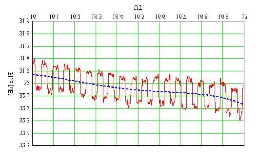
ETH Zürich RADIO ASTRONOMY AND PLASMA PHYSICS GROUP
to be explored and as far as possible to be taken into account within the evaluation of the final
result.
2. Measuring equipment
The main part as already mentioned is a complete low cost satellite receiving system bought
from a super market here in Zürich. Its low noise figure (NF) according to the specification is
better than NF=0.9dB (noise figure) corresponding to Tsys=70 Kelvin excess noise at room
temperature. This is more than 100 times better than the receiver of Dicke and Beringer. The
parabola mirror together with the LNC (low noise converter) is mounted saprophytically on
the western rim of the 5m parabola antenna of the IFA (Institute of Astronomy) of ETH
Zürich [3]. This mounting method allows controlling the position electronically by a standard
personal computer in particular to follow the path of the moon from moon-rise to moon-set.
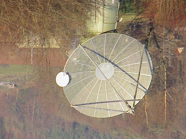
Fig. 1: 80cm satellite antenna mounted on a 5m dish antenna at Bleien observatory. The
observatory with receiver and computers is 50m to the right side of the tower.
The personal computer can be monitored remotly and controlled via VNC (virtual network
computing). Thus it is very easy to do the controlling functions in a comfortable way from my
home. The computer does not only track the moon, but it also offers the method of beam-
switching, a very efficient method to measure small flux changes on a warm or even hot
background noise level. The LNC is powered with a bias-T, feeding U=+15Volts direct
current from the observatory's power supply. The frequency-depending attenuation of the 50m
long cable between LNC and receiver is flattened by an ordinary TV-equaliser. The satellite
IF (intermediate frequency) of 950MHz to 1.95GHz is then fed into a standard
communications receiver AR5000 to select the desired receiving frequency, to amplify the
noise signal and to limit the observing bandwidth to B=220KHz or even less. A broader
bandwidth is quite desirable, but the interference from geostationary satellite communication
signals would increase drastically. The second IF of 10.7MHz is directly fed to a logarithmic
detector AD8307 of Analog Devices with a conversion constant of k=25mV/dB. The
analogue output of the logarithmic detector is directly measured with a standard bench digital
multimeter FLUKE45. The RS232 output of the multimeter is fed to the communication port
COM1 of an additional personal computer. It reads the serially sent data and stores them on
Page: 2/11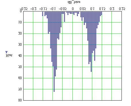
ETH Zürich                                 RADIO ASTRONOMY AND PLASMA PHYSICS GROUP

harddisk in ASCII format where each entry represents the radio flux expressed in volts.
Subsequently the locally stored data can be transferred to my home or to the IFA via ftp.

3. Measuring methods

3.1 Frontend

It is common knowledge that the background temperature of the sky is a non-linear function
of the telescopes elevation. Thus a method is needed to compensate varying background noise
levels. I use a beam switching method to compensate the influences of high background noise
at low elevation wich is similar to the method Dicke used 55 years ago The switching phase
stays ∆t=90 seconds on source, changes as fast as possible by ∆α=6 degrees eastward to the
source for another ∆t=90 seconds. This sequence is automatically repeated as long as the
moon is above the horizon in Bleien. The switching time of ∆t=90 second has to match with
integration time and drifting variations due to temperature variations either of the LNC or of
the receiver detector system. The nominal switching time has to be higher than the integration
time but has also to be shorter than any drifting component in the whole system; thus in my
configuration ∆t=90 seconds is a good compromise. The deflection angle of ∆α=6 degrees is
another compromise. It has to be larger than the beam angle of the telescope, but it should be
as small as possible to not waste useful measuring time, because after all the antenna control
system needs a couple of seconds to reach the deflection of ∆α=6 degrees.

Fig. 2: Hardware structure of the radio astronomy receiving system from antennae (left) via
receiver to the personal computer (right).

3.2. Backend

The collected data are visualised every day after transferring them to my home computer. The
data (ASCII-files) can be visualised with EXCEL, MATH-CAD, MAT-LAB or any other
spreadsheet program. Every file has to be identified with the correct starting time in UT that is

                                           Page: 3/11
ETH Zürich RADIO ASTRONOMY AND PLASMA PHYSICS GROUP
delivered through a professional GPS system from within the observatory. The data usually
are split into subsequent files of 1 hour duration, 900 measurement points each, making the
analysis on PC level simpler. The mean elevation ε of the telescope has to be calculated to
compensate the atmospheric attenuation for every file with 1 hour duration. For correlation
purposes and for visualisation processes I also need the moon phase angle φ, the moon disk
diameter Φ and the illumination factor ξ. These values are automatically calculated by a home
brewed Windows application program according to date and time UT (universal time). To
calculate the antenna temperature it is necessary to know the proper reference temperature
Tref. In my configuration (as a first approximation) I decided to use the temperature of the
logarithmic detector in the observatory Tref=Trx (rx = receiver). This temperature can be
copied free from the environmental data file yyyymmdd.wdf of the Phoenix-2
radiospectrograph at Bleien observatory. The datafile is stored once per day and can be
viewed with any browser on http://www.astro.phys.ethz.ch/rapp/. The temperature Tlnc of the LNC
can also be picked out of the weather data file also with a time resolution of 1 minute.
Fig. 3: Evaluation of mean moon flux in decibels using a fitting function to split background
flux and moon flux. The slow variations are due to different elevation angles, temperature
changes of LNC and/or changes in receiver stability. The solid red curve is subtracted from
the blue dotted fitting curve. Statistical analysis (median value) of the difference pattern
results in a single flux value for that file of February 16, 2001. The fitting curve is chosen in
such a way that the residual dispersion or variance is a minimum. In that special case a 4th
order polynom was chosen.
Page: 4/11ETH Zürich RADIO ASTRONOMY AND PLASMA PHYSICS GROUP
Fig. 4: Histogram of the data file of Fig. 3 above. The left peak represents the noise
distribution of the background radiation only, while the right peak represents the background
noise plus the excess noise distribution of the moon. The difference between both peaks is
stored as a single value expressed in decibels. Here in this example, I got 0.197dB
corresponding to an antenna temperature of about 4.4 Kelvin at an average system
temperature of 94 Kelvin.
3.3 Analysis steps
3.3.1 Exception handling
Prior to analysis the data has to be checked for plausibility. There are a huge number of
interference possibilities. All data with non-expected data were deleted, especially all with a
dispersion larger than 40 Kelvin. There are several days with really exotic conditions where
no useful data can be recorded. On January 15, 2001, for example, the moon was hidden by
the geostationary satellite path and thus the strong radio flux saturated the receiving system;
no measurement was possible. Another critical date was January 24, 2001, when the sun and
moon both had similar sideral coordinates (new moon). The sun outshines the moon several
thousand times; thus no measurements were possible at all. Measurements near the horizon
are often critical because of the high background temperature (300 Kelvin) or due to
interference by man made noise. Another critical point was found during the experiments
while using beam switching mode. Our beam switching method first worked only in
horizontal (azimuthal) direction. As soon as the moon is higher than 45° above the horizon,
the horizontal deflection is really unsuitable because the deflection angle on the sky is
reduced due to cosine(elevation) effect. If I observed in zenith, the deflection angle would be
exactly zero and we would only rotate the polarisation plane of the LNC. Therefore I
introduced another option within the on/off-source method. Now I can select between
horizontal or vertical deflection. Vertical deflection is not influenced by cosine(elevation) but
Page: 5/11ETH Zürich RADIO ASTRONOMY AND PLASMA PHYSICS GROUP
it is only allowed for elevations larger than 30°. Otherwise the antenna would point to the
horizon every time and would therefore increase the system noise. All non-exceptional data
are analyzed by the following procedures.
3.3.2 Analysis
The stored data first has to be converted into equivalent antenna temperature using an
estimation of the reference temperature Tref. Due to missing calibration sources, Tref was
calculated by three different methods. The first method uses the noise figure NF of the LNC
plus internal losses of dust cover plus atmospheric attenuation plus sky background
temperature which leads to about 89 Kelvin. The second method uses a back-tracking
calculation of the solar radio noise measured at NOAA which leads to 90 Kelvin. And the
third method uses the ambient temperature of the horizon (forest) at Bleien observatory which
leads to about 104 Kelvin. I then took the average value of the above three different methods
to Tref = 94 Kelvin.
RFdB
Ta = Tref ⋅ 10 10 dB − 1 (1)
This calculated antenna temperature is too low because of several more or less exactly known
attenuation coefficients. The first not yet exactly known attenuation coefficient is the
attenuation γc of the dust cover of the LNC. It can only be measured by killing the device. I
definitely not like that method, though I took an estimation obtained from colleagues and
from experience with other LNC's. One can assume that the attenuation is in the range of
0.1dB to 0.3dB, here I have decided to use 0.1dB. The end result can be corrected as soon as
the dust cover can be measured.
0.1dB
γc = 10 10 dB
(2)
Now we can calculate the antenna temperature of the moon on the earth but that's still not the
proper value because the atmosphere has an attenuation of at least aa=0.22dB in zenith. The
value varies with different authors from 0.20dB to 0.24dB and for rainclouds even up to
1.5dB. I have decided to use the more pessimistic value of aa=0.22dB. Unfortunately I never
measured the moon in zenith, thus one has to take into account the non-linear increase of the
attenuation for other elevations than zenith. Several papers have been published dealing this
topic. The air at the horizon is thicker than in zenith thus the attenuation near the horizon is a
maximum. The attenuation of the radiation due to the atmospheric absorption will decrease
the measured flux of a radio source. If S(z) is the flux measured at zenith distance z, and So is
the flux that would be obtained outside the atmosphere, then
S ( z ) = So ⋅ aa − X ( z ) (3)
where aa is the atmospheric attenuation at the zenith for the airmass 1, and X(z) is the relative
airmass in units of the airmass at the zenith. For a plane parallel atmospheric model clearly
follows
Page: 6/11ETH Zürich RADIO ASTRONOMY AND PLASMA PHYSICS GROUP
1
X ( z ) = sec( z ) = (4)
cos( z )
Schönberg 1929 [7] has done extensive investigations of X(z), a Chebyshev-fit to these data
up to X=5.2 with an error of less than 1promille is given by
1.00672 0.002234 0.0006247
X ( z ) = −0.0045 + − − (5)
cos( z ) cos( z ) 2 cos( z ) 3
For my own calculations I decided to use the simpler version according to (4). Applied to my
configuration an atmospheric correction coefficient γa can be calculated by
π
sin(ε ⋅ ) −1
γa = aa 180
(6)
According to Kraus [3] one has also to take into account the shape of the antenna to calculate
the proper antenna temperature. Depending on form, size and shape of the antenna he
proposes a shape factor κ which in my configuration is about κ=1.02±0.05
All correction factors now can be combined into an overall loss factor γ.
γ = γc ⋅ γa ⋅ κ (7)
Now we are able to calculate the proper antenna temperature Tp as a basis to estimate the
final moon temperature.
Tp = Ta ⋅ γ (8)
The calculation of the moon temperature requires to know the beam geometry as exactly as
possible. Several methods to evaluate the beam angle are known. I decided to measure the
beam parameters by a meridian transit measurement of the sun on January 12, 2001 at a
declination of δ=-21.6°. The normalisation and integration of the sun's transit data leads to the
so-called directivity D, but unfortunately only for one polarisation. The data couldn't be
integrated in a closed form thus I had to do it with the Σ-operator. First we need the radio
signal of the sun not in decibels but in physical units e.g. in Kelvin antenna temperature.
RFdB
RF = 300 K ⋅ 10 10 dB − 1 (9)
Then we have to normalise the antenna temperature pattern between 0 and 1.0
RF − min( RF )
RFn = (10)
max( RF ) − min( RF )
Page: 7/11ETH Zürich RADIO ASTRONOMY AND PLASMA PHYSICS GROUP
The analysis of that normalized power pattern leads directly to the half power beam width
HPBW
360° π
HPBW = 0.192h ⋅ ⋅ cos − 21.6° ⋅ = 2.88° (11)
24h 180°
This normalised radio frequency power pattern on the other hand now can be summed up to S
with
S = ∑i RFn ⋅ δα (12)
where
4 sec/ sample 360°
δα = ⋅ = 0.017° / sample (13)
3600 sec/ h 24h
Now the directivity D can be quantified to
2
180°
4 ⋅π ⋅
π
D= = 4478 (14)
S2
The directivity D can easily be converted into antenna gain G which can be compared with
other measurement methods.
G = 10 ⋅ log( D) = 35.6dB (15)
Again according to Kraus [3], D can directly be converted into the interesting beam solid
angle Ωa, expressed in square degrees.
4 ⋅π
Ωa = 2
= 9.212 (16)
π
D ⋅
180°
On the other hand the apparent diameter Φ of the observed moon is not constant. During a
moon phase angle φ it varies several percent. The more than three hundred individual values
were calculated numerically and so the moon solid angle Ωm expressed in squre degrees can
be estimated by
2
Φ
Ωm = π ⋅ (17)
2
All components (1) until (17) are now known to finally calculate the moon's temperature Tm
as a function of antenna temperature, system temperature, elevation, losses, beam angles and
so forth.
Ωa Page: 8/11
Tm = Tp ⋅ (18)
ΩmETH Zürich RADIO ASTRONOMY AND PLASMA PHYSICS GROUP
Tm (18) is the brightness temperature at 2.77cm wavelength averaged over the moon's disk
and will be referred to as disk temperature.
4. Results
After doing all mathematis given in (1) to (18) we get a viewgraph of the moon's temperature
Tm as a function of moon phase angle φ. The dark blue dots represent the moon temperature
Tm, while the solid thick red line represents a 6th order polynom filtered approximation of all
data. The polynom filter removes the noisy high frequency part of the curve and smoothes it.
The deviation 1σ is less than 10 Kelvin (1σ < 4% of mean disk temperature) while the mean
value is about 213 Kelvin. One can easily recognise the phase lag of the maximum
temperature with 236 Kelvin of nearly 5 days after full moon and a minimum temperature of
about 192 Kelvin 2 days prior to full moon.
Moon Surface Temperature @ 2.77cm
300
280
260
Temperature [Kelvin]
240
220
200
180
160
140
120
New Full New
100
0 30 60 90 120 150 180 210 240 270 300 330 360
Phase angle [°]
Fig. 5: Moon's disk temperature at 2.77cm wavelength versus moon phase angle φ during two
complete cycles from twice new moon via full moon to new moon again.
5. Conclusions
Page: 9/11ETH Zürich RADIO ASTRONOMY AND PLASMA PHYSICS GROUP
I have shown that it is possible to repeat classic astronomical experiments [8] with rather
simple and/or cheap hardware. Satellite LNAs nowadays have such a low system temperature
that it might even be possible to detect other planets of our solar system by using adequate
measuring methods, integration time and bandwidth. In the above experiment to measure the
moon's disk temperature a better sensitivity could be achieved with higher integration time
and/or higher bandwidth. An explanation for the higher time lag in comparison with other
authors is not yet clear. Dicke and Beringer measured a time lag of about 3 days after full
moon at a wavelength of 1.25cm. In my case (5 days after full moon), I assume that at longer
wavelength of 2.77cm the time lag must be larger due to the simple fact that the longer the
wavelength the deeper is the penetration of the electromagnetic waves into the dust of the
moon's surface. The measurement methods can be optimised using a calibrated and thermal
controlled low noise converter to reduce systematically errors. An integration circuit would
reduce system noise and increase the overall sensitivity drastically. Sampling data at a higher
sampling rate would allow to improve statistical errors even more. More measurements
should be done at the same frequency to confirm my own measurements. On the other hand, it
would make sense to repeat all measurements at different frequencies to confirm the
dependency of time lag on frequency. These experiments havn't been done for several years.
Mankind's interest for the physical behaviour of our moon has been lost since Apollo 11, but
it should be increased again. The latest paper published by Jaime Alvarez-Muñiz and Enrique
Zas [9] shows that the moon comes into interest again as a very large detector for cosmic
particels and neutrons. Radio observations of the whole moon may become of primary interest
to physicists.
Acknowledgements. Herewith I thank Michael Arnold for upgrading the antenna control
software to observe non-solar sources in on/off-source mode. I also thank Ken Becker for
checking and correcting my English text. Electrical power, observation time and some
network bandwidth was liberally spent by IFA ETH Zurich.
References
[1] Dicke, R. H. and Beringer, R., 'Microwave radiation from the sun and the moon',
Astrophys. J. 103, 375
[2] Piddington, J. H. and Minnett, H. C., 'Microwave thermal radiation from the moon', Aust.
J. Sci. Res. A2, 63.
[3] John D. Kraus, Radio Astronomy, McGraw -Hill Book Company, New York 1966, ISBN
07-035392-1
[4] J. S. Hey, Das Radiouniversum, Einführung in die Radioastronomie, Verlag Chemie,
Weinheim 1974, ISBN 3-527-25563-X
[5] J. S. Hey, The Evolution of Radio Astronomy, Elek Science, London 1973, isbn 236-
15453-2
[6] Astronomical Institute ETH Zürich, Scheuchzerstrasse 7, CH-8092 Zürich,
http://www.astro.phys.ethz.ch/rapp/
Page: 10/11ETH Zürich RADIO ASTRONOMY AND PLASMA PHYSICS GROUP
[7] Schönberg E. (1929): Theoretische Photometrie, Handbuch der Astrophysik Bd. II/1 ed.
by K. F. Bottlinger et al. (Springer Berlin)
[8] Woodruff, Turner, Sullivan: Classics in Radio Astronomy, D. Reidel Publishing
Company, Dordrecht Holland 1982, isbn 90-277-1356-1
[9] Jaime Alvarez-Muñiz, Enrique Zas: Prospects for radio detection of extremely high energy
cosmic rays and neutrinos in the moon. New Scientist (Nr. 2280, p.7) 3 March 2001. More at:
http://xxx.lanl.gov/abs/astro-ph/0102173
Page: 11/11You can also read