The neuronal basis of spontaneous flight behavior in Drosophila
←
→
Page content transcription
If your browser does not render page correctly, please read the page content below
The neuronal basis of spontaneous flight

                          behavior in Drosophila

Inaugural-Dissertation to obtain the academic degree Doctor
             rerum naturalium (Dr. rer. nat.)
  submitted to the Department of Biology, Chemistry and
          Pharmacy of Freie Universität Berlin

                            by
                   Sathishkumar Raja

             From Namakkal 11°13′N 78°10′E

May, 2013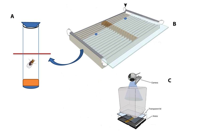
Ph.D. Dissertation Supervisor – Dr. Björn Brembs,

Institut für Biologie - Neurobiologie,

Freie Universität Berlin.

2010 – 2013.

1st Reviewer: Prof. Dr. Björn Brembs

2nd Reviewer: Prof. Dr. Hans-Joachim Pflüger

Date of defence: 13/06/2013

2|Page
DEDICATED TO TRUE FLIES….

3|Page

TABLE OF CONTENTS:
1 INTRODUCTION ...................................................................................................... 7

  1.1 NEURONAL BASIS OF VISUALLY GUIDED BEHAVIORS ................................................ 8
  1.2 NEURONAL CAUSES FOR SPONTANEOUS BEHAVIORAL VARIABILITY .......................... 9
     1.2.1 Spontaneous occurrence of animal behavior and its variability ................... 9
     1.2.2 Variability in behavior is an adaptive trait .................................................... 9
     1.2.3 Intrinsic neuronal properties for spontaneous variability ........................... 10
  1.3 NEUROETHOLOGICAL APPROACH TO NEURONAL CIRCUIT INVESTIGATION .............. 12
     1.3.1 Endogenous flight behavior of Drosophila as measured by a wing beat
     analyzer ................................................................................................................... 12
     1.3.2 Dissection of neuronal circuits using the Gal4-UAS system coupled with a
     tetanus toxin light chain (TeTxLC): ....................................................................... 13
     1.3.3 A dynamic systems approach for investigating neuronal circuits ............... 15
  1.4 A STRATEGY TO ESTABLISH THE LINK BETWEEN A NEURONAL CIRCUIT AND
  SPONTANEOUS BEHAVIORAL GENERATION                             ................................................................... 16

2. MATERIALS AND METHODS ............................................................................ 18

  2.1 FLIES ..................................................................................................................... 18
  2.2 SPONTANEOUS YAW TORQUE MEASUREMENT ......................................................... 19
     2.2.1 Tethering flies for yaw torque measurements ............................................... 19
     2.2.2 Optical wing-beat analyzer ............................................................................ 19
     2.2.3 Signal optimization ....................................................................................... 22
  2.3 MODULAR DISPLAY SYSTEM ................................................................................... 23
  2.4 ANALYSIS OF YAW TORQUE DATA ............................................................................ 26
     2.4.1 Fast Fourier Transform (FFT) ...................................................................... 26
     2.4.2 S-Map procedure ............................................................................................ 27
     2.4.3 Spike detection algorithm .............................................................................. 30
     2.4.4 Geometric Random Inner Product (GRIP) analysis ..................................... 30
  2.5 THE BURIDAN PARADIGM....................................................................................... 31

4|Page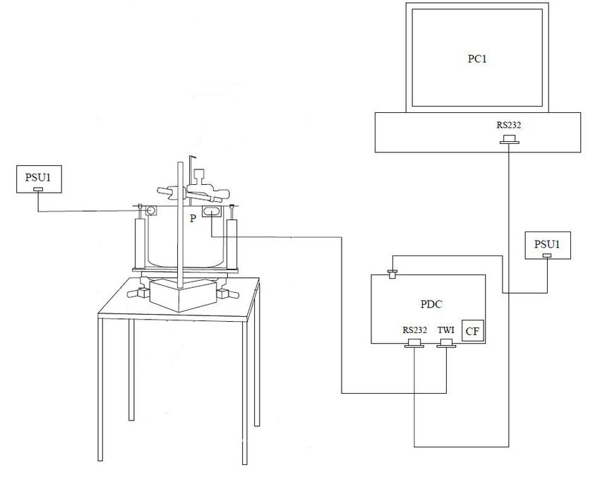
2.5.1 Flies ................................................................................................................ 31
     2.5.2 Hardware components ................................................................................... 31
     2.5.3 Tracking software BuriTrack ........................................................................ 32
     2.5.4 CeTrAn Centroid Trajectories Analysis software ......................................... 33
     2.5.5 General activity measurement ....................................................................... 33
     2.5.6 Inter-activity interval extraction ................................................................... 34
  2.6 PYSOLO ASSAY ....................................................................................................... 34
     2.6.1 Flies ................................................................................................................ 34
     2.6.2 Hardware components ................................................................................... 35
     2.6.3 Configuration ................................................................................................. 35
     2.6.4 Midline crossing events ……………………………………………………………………….36
  2.7 FLY SIESTA AND BURSTINESS ANALYSIS ................................................................ 37
  2.8 STATISTICAL ANALYSIS .......................................................................................... 38

3. RESULTS................................................................................................................ 39

  3.1 NO-NOISE FREQUENCY COMPONENTS FROM THE WING BEAT ANALYZER ................. 39
  3.2 S-MAP ANALYSIS CAN BE USED WITH VARIABLE FLIGHT DURATION ........................ 41
  3.3 SCREENING FOR NEURONAL CANDIDATES THAT GENERATE LINEAR SIGNATURES IN
  S-MAP ANALYSIS .......................................................................................................... 43
  3.4 LINEAR STRUCTURE IN S-MAP ANALYSIS FROM DOUBLE C232; C105-GAL4 CAUSED
  BY TETANUS TOXIN EXPRESSION................................................................................... 44

  3.5 NEURONAL ORGANIZATION FOR NONLINEARITY GENERATION ................................ 46
  3.6 LOCOMOTOR COMPETENCE OF CANDIDATE FLY LINE .............................................. 47
     3.6.1 Measurement of yaw torque spikes ................................................................ 48
     3.6.2 Walking Activity measurement...................................................................... 49
     3.6.3 Inter-event interval distribution analysis ..................................................... 50

4. DISCUSSION .......................................................................................................... 53

  4.1 NEURAL CIRCUITRY UNDERLYING SPONTANEOUS BEHAVIORAL VARIABILITY ......... 53
     4.1.1 Ellipsoid body ring neurons mediate the nonlinear structure in spontaneous
     flight behavior

5|Page
4.1.2 The temporal pattern of spontaneous behavioral variability and its
     independence from associated locomotor activity .................................................. 54
  4.2 FUNCTIONAL NEURONAL ARCHITECTURE FOR NONLINEAR STRUCTURE GENERATION
   .................................................................................................................................... 57
  4.3 LEVEL OF BRAIN ORGANIZATION: CONNECTING ENDOGENOUS FLIGHT BEHAVIOR
  WITH INTRINSIC BRAIN ORGANIZATION ......................................................................... 58

  4.4 FUTURE OUTLOOK: DO NONLINEAR CIRCUITS CONTROL OPERANT ACTIVITY
  INITIATION?        ................................................................................................................. 59

5. SUMMARY: ............................................................................................................. 61

6. BIBLIOGRAPHY: ................................................................................................ 64

7. ACKNOWLEDGEMENT: ...................................................................................... 74

6|Page
1 INTRODUCTION
Brain function is primarily studied by observing correlations between
behaviors and environmental events. Behavioral responses are considered to be
stereotypic patterns of reflexes driven by immediate environmental stimuli. This
view can be traced to the early work of Sherrington (Burke, 2007; Levine, 2007;
Sherrington, Charles Scott, Sir, 1920), who emphasized the role of sensory inputs on
reflexive behavior. This finding stimulated a number of studies, on animals from
single cell organisms (Jimenez-Sanchez, 2012) to humans (Churchland et al., 2010;
Müller et al., 2013; Sommer et al., 2013), that were designed on the assumption
that external cues elicit appropriate responses or, stated another way, that brain
function is best understood in terms of input-output transformations (Borst &
Egelhaaf, 1989; Borst & Bahde, 1988; Dickinson et. al 2013; Huston & Jayaraman,
2011; Maimon & Dickinson, 2010; Murray & Wallace, 2011; Wessnitzer & Webb,
2006).
For example, behavioral studies of insects are conducted by manipulating
various stimuli that are known to cause behavioral responses. Insects have several
sensory modalities that receive external cues and relay relevant information to
central processing circuits for successful motor output (Dickinson, 2005; Frye &
Dickinson, 2004). The major sensory modalities of insects are olfaction, taste,
mechanoreception and vision. These have been studied extensively using
behavioral, genetic and neurophysiological methods. (Frye et al., 2011; Götz, 1987;
Borst et al., 2011; Nachtigall & Wilson, 1967; Renn et al., 1999). This behavioral
research illuminates brain function by focusing on the neural mechanisms of insects
that process sensory stimuli to produce complex behaviors (Comer & Robertson,
2001; Renn et al., 1999; Strauss, 2002; Venken, Simpson, & Bellen, 2011).
7|Page1.1 Neuronal basis of visually guided behaviors
Most of the behavioral studies of insect flight have been conducted by
presenting visual stimuli in the form of gratings (Borst & Bahde, 1988; Tammero &
Dickinson, 2002). Flies are better able to abstract fast-moving stimuli than many
other species. Tethered flight studies are conducted in a flight simulator where the
flies are partially immobilized in the center of a panorama on which visual cues are
projected (Götz, 1968; Frye et al., 2008; Wang et al., 2008; Wolf & Heisenberg, 1980;
Reinhard Wolf & Heisenberg, 1991). Studies involving free and tethered flight have
successfully addressed the underlying neuronal processes governing visual-motor
transformation during such events as obstacle avoidance (Horridge, 2009; May,
2012), object discrimination ( Borst & Egelhaaf, 1989; Comer & Robertson, 2001;
Griffith, 2012) and escape behavior (Card & Dickinson, 2008; Conner & Corcoran,
2012; Dewell & Gabbiani, 2012; Domenici, Blagburn, & Bacon, 2011; Roeder, 1962).
These studies have shown that a visual cue that reaches the visual system is
encoded, processed through central circuitries, integrated by mechanosensory
feedback, and finally transformed into a specific flight maneuver (Borst & Haag,
2002; Frye & Dickinson, 2004). The pathways that route visual information toward
descending interneurons have been studied extensively ( Borst & Egelhaaf, 1989;
Borst & Reiff, 2010; Borst, 2009; Collett, 2002; Götz, 1968; Jung et al., 2011; Gong &
Liu, 2012). These descending interneurons are believed to carry stimulus
information from sensory units that is essential for flight motor circuitry (Maimon
et al., 2010). However, the mechanism involved in triggering motor patterns by
central circuitry is largely unstudied.
It has been shown that fast-moving cues are recognized by a set of wide- and
small-field neurons. These neurons are specialized cells that detect the direction of
motion and the movement of a small object against its background (Card &
Dickinson, 2008; Borst, & Haag, 2005). A pair of large-diameter interneurons,
known as giant fibers, mediate the fast motor responses that initiate fly escape
sequences (Card & Dickinson, 2008; Wyman, 2013). The relationship between
8|Pageidentified neurons and behavior is ultimately established by observing sensory-
motor processing. Such findings support the assumption that control of the motor
units involved in any flight behavior is stimulus-regulated and eliminate the
possibility of endogenously generated motor actions.
1.2 Neuronal causes for spontaneous behavioral variability
1.2.1 Spontaneous occurrence of animal behavior and its variability
Spontaneous behavior is ubiquitous in several biological systems (Miller,
1997; April, 1970). The movement dynamics of many animals show relatively
variable and spontaneous behavior. The copepod Temora longicornis Müller is a
small crustacean that floats on water and feeds on unicellular algae. Copepods
initiate movement toward the algal rich zone, but when they are reared in a lab
environment providing no algae in the water, they travel in a straight line with
interspersed spontaneous quick turns (Schmitt & Seuront, 2001). This is considered
to be a spontaneous exploratory movement. The giant water bug Belostoma
flumineum displays alternation between left and right turns in a T-maze in a
seemingly random fashion. Goldfish switch between a slow and quick swimming
pattern in a uniform visual environment. Most importantly, the duration of the
activity is variable (Nepomnyashchikh, 2013).
1.2.2 Variability in behavior is an adaptive trait
Spontaneous behavior generated by animals is highly variable (Maye et al.,
2007; Nepomnyashchikh & Podgornyj, 2003). It is therefore difficult to predict every
move that an animal will make. It has been suggested that brains have evolved over
time to generate unpredictable adaptive variability in behaviors such as those
involved in competition, courtship and chasing (Nepomnyashchikh & Podgornyj,
2003; Nepomnyashchikh, 2013; Wilkinson, 1997). This view began with the
‘Machiavellian Intelligence’ hypothesis, which states that animals and humans
developed specific cognitive skills for predicting and manipulating the actions of
other beings. Individuals have developed a protean strategy to prevent other
9|Pageanimals from successfully predicting their behavior (Miller, 1997; April, 1970).
Behavior that is unpredictable favors survival and is thus adaptive. These
unpredictability strategies were first identified in the 1960s, in studies of the escape
strategies of moths and the facultative defensive behaviors of rats (Chance, 1957).
Moths execute combinations of loops, rolls, and dives to evade bats ( Roeder, 1964;
Roeder, 1962). Rats randomly exhibit convulsions upon hearing noxious tones.
These behaviors would confound a predator and make it more difficult for it to catch
prey. If animals actions were automata, every action would be released by a
stimulus that determines behavior (Wilkinson, 1997).
These examples of predator-prey interaction show that unpredictable
behavior is certainly advantageous for survival. Consistency in stereotyped predator
avoidance responses would make prey more vulnerable. Unpredictability is not
limited to predator-prey interactions. Variability also maintains orderly behavior at
several levels of animal organization. Some examples are posture maintenance
(Oullier, Marin, & Stoffregen, 2006), landing on objects (Saint-germain, Drapeau, &
Buddle, 2009) and perceptual scanning (Estes, 1965). Variability is utilized at
several levels of physiological organization. Complex behavioral repertoires are
developed by reinforcement of behavioral variants, for example in random
exploratory behavior (Miller, 1997). Nevertheless, unpredictability is observed in
animal actions, movement signals, and social interactions. However, variability
could be highly disadvantageous if it is entirely randomly generated. Prey could be
falling directly on top of a predator during truly random predator avoidance.
1.2.3 Intrinsic neuronal properties for spontaneous variability
Evolution is largely assumed to produce deterministic mechanisms of animal
behavior. Unpredictability is disregarded as a noisy component according to the
computational principles of the input-output hypothesis (Selen & Wolpert, 2008;
Series & Note, 2000; Gossen, & Jones, 2005). The sensorimotor integration principle
also does not provide a sufficient interpretation of the spontaneous behavioral
variability that occurs in a wide range of species. Brain functions are complex, and
10 | P a g estudies of sensorimotor integration have not produced a complete picture of brain
function. To the best of our knowledge of brain structure, function arises through
the transmission of information from sensory to motor networks. Variability thus
does not arise from completely random or chance components in the brain. The
combination of inevitability (e.g., primary goal, escape) and variability favors
unpredictable behavior. The precision of the required behavior is largely dependent
on the needs of an animal in a particular environment. Neuronal circuits in the fly
brain are proposed to mediate such organized behavioral architecture (Maye et al.,
2007).
In higher-order brain systems, spontaneous activity occurs at the neuronal
level (Andrews-Hanna et al., 2008; He et al., 2010; Proekt, Banavar, Maritan, &
Pfaff, 2012; Raichle, 2010). Variability in the timing of evoked neuronal spiking is
reported as well. This variability in the timing of neuronal firing is associated with
spontaneous brain activity. Specific neuronal networks called default mode
networks (DMNs) have been shown to interact and thus induce brain activity
(Raichle, 2010). This interaction is a primary cause for variability in the human
brain. However, a direct comparison with invertebrate brain structures is not
productive given the huge gap in brain complexity. However, Drosophila and
humans share certain brain properties, as evidenced by similarities in mediating
action selection and time allocation by the insect and human brains (Van Alphen, &
Pierre, 2010; Reiter & Bier, 2002).
Maye et al., 2007 proposed a neuronal cause for spontaneous variability after
investigating the temporal structure of behavioral variability in Drosophila.
Restrained Drosophila can spontaneously produce yaw torques in a flight simulator
with no visual cues that could potentially elicit turning responses (Maye et al.,
2007; Wolf and Heisenberg, 1984). The yaw torque generated spontaneously by the
flies is highly variable, with random alternation between left and right turns. These
actions are proposed to be dependent on active and voluntary brain activities (Maye
et al., 2007). The interval between alternating turns shows a fractal order
11 | P a g eresembling levy flights, suggesting the role of initiation by an endogenous neuronal
entity(ies). This endogenous neuronal entity is proposed to act as a deterministic
system to keep variability under neural control.
The few studies of endogenous animal behavior highlight some yet-
unanswered ultimate questions, such as ‘Is there a neural entity mediating such
processes with negligible external cues?’ and ‘If so, how is the endogenous
generation of spontaneous variability in Drosophila organized without external
input?’
1.3 Neuroethological approach to neuronal circuit investigation
1.3.1 Endogenous flight behavior of Drosophila as measured by a wing beat
analyzer
In general, measuring endogenously generated motor output is required for
finding the neuronal causes of spontaneous behavior. External cues should have
minimal or no influence over the measured output. Flight simulators have been
used for several decades to measure visual-motor responses in a controlled
environment. Flight simulators have been used widely to study such topics as visual
motion detection, visual learning, orientation, reafference controls, and optomotor
responses (Brembs, 2002; Liu et al., 2006; Wolf & Heisenberg, 1991). Display
systems that are based on light-emitting diodes (LEDs) (Reiser & Dickinson, 2008)
have recently been used to display panoramic visual motion at high spatial and
temporal resolution. The inter-ommatidial distance of the Drosophila eye is more
than the individual pixel size of an LED display unit (Chow et al., 2011; Mamiya &
Dickinson, 2011; Reiser et al., 2011). The fly retina is thus able to detect any minute
spatial movement in an arena. For spontaneous behavioral studies, flies are
tethered and the flight arena is programmed to display a uniform, unchanging
display environment. The feedback loop between the behavior and the environment
is open. This uniform environment is suitable for measuring endogenous flight
behavior because it excludes external stimuli. Drosophila can fly under these
12 | P a g econditions, and the wing beat amplitude is measured for computing yaw torque.
Tethering also limits the fly’s mobility, but this procedure offers several advantages
in addition to environmental control. For example, because the tethered flies have
no spatial movement, there can be no angular rotation feedback to the flight motor
center such as that from halters (Chow et al., 2011; Huston & Krapp, 2009;
Sherman, 2003).
The electronic visual flight arena and the wing beat analyzer have proven to
constitute a suitable system for delivering controlled visual stimuli and measuring
yaw torque motor output (Dickinson, 2005; Dickinson, 1993; Reiser & Dickinson,
2008). The optical sensor-based wing beat analyzer measures the wing beat
amplitudes of individual wings. The left and right wing beat amplitude difference is
equivalent to a yaw saccade turn detected during free flight. This yaw torque
measurement under homogenous spatial scenery is used as a measure of
endogenous motor output production. Therefore, yaw turning actions generated by
the flies are not triggered by visual cues, and any modulation in yaw turning
originates intrinsically from the fly brain.
1.3.2 Dissection of neuronal circuits using the Gal4-UAS system coupled with a
tetanus toxin light chain (TeTxLC):
A noninvasive targeted expression tool known as the Gal4-UAS tool system is
widely used to identify the causal neuronal bases of a specific behavior (Duffy, 2002;
Martin & Sweeney, 2002; Renn et al., 1999; Venken et al., 2011). The basic concept
of this system is accessing a behavioral function in the absence of a specified
neuronal population to determine the causal circuitries by elimination. This system
allows the expression of a gene of interest in any neuronal cell or group of tissues.
For example, the tetanus toxin light chain (TeTxLC) is widely used to investigate
the role of a particular brain region on a specific behavior. The usefulness of this
approach is due to the mechanism and action of the tetanus toxin light chain. The
light chain inhibits exocytotic neurotransmitter release by proteolytically cleaving a
protein called synaptobrevin. Synaptobrevin (Sweeney et al., 1995) is found to
13 | P a g einteract with presynaptic proteins to mediate an evoked transmitter release by
effectively silencing the neuronal region affected by this toxin. This concept has led
to the identification and molecular characterization of several neuronal bases and
associated pathways in olfaction, mechanoreception, higher order locomotion and
vision in fruit flies.
Fig. 1. The Gal4-UAS system.
This figure depicts the working principles of
Gal4-UAS system. Effector lines consist of a
Gal4-binding upstream activation sequence
(UAS) with the sequence of the gene of interest
(tetanus toxin gene). In UAS-TNT-E flies, the
tetanus toxin light chain gene is placed next to
UAS elements. The toxin is only expressed in
cells of the progeny that express Gal4 (adapted
from Griffith, 2012).
The Gal4-UAS system is used to express tetanus toxin into the neural cells.
Gal4 is a transcriptional activator protein that activates transcription in the yeast
Saccharomyces cerevisiae induced by galactose. Gal4 directly binds to a defined site,
called the "Upstream Activating Sequence" (UAS) and has no target in the fly
genome. The tool uses a transposable "P-element" construct that can be inserted
into the fly genome at different sites. The P-element contains the Gal4 sequence
14 | P a g ewith either a known promoter (promoter-fused Gal4 lines) or a weak promoter that
will "trap" enhancers close to the insertion site (enhancer trap line) (Brand &
Perrimon, 1993). GAL4, in turn, directs the transcription of the GAL4-responsive
UAS target gene in an identical pattern. This bipartite approach, which uses two
separate parental lines, i.e., the driver (Gal4) line and the effector (UAS) line, has a
major advantage: the ability to target the expression of any effector gene in a
variety of spatial and temporal ways by crossing it to distinct Gal4 drivers. Wide
ranges of Gal4 driver fly lines are available commercially with expression patterns
ranging from a group of cells to entire brain regions.
1.3.3 A dynamic systems approach for investigating neuronal circuits
There is spontaneity in a given system that is independent of the stimulus. A
stimulus-behavior unit is a deterministic linear system when a sensory stimulus
triggers central circuitries and directly facilitates the resulting behavior. However,
spontaneity is manifested in a nonlinear dynamic system. The system with
spontaneous behavior is said to be a nonlinear dynamic system because the
behavioral actions are not specifically proportional to the external sensory
parameters. This endogenously generated behavior could have an unpredictable or
deterministic nature and reflects the nonlinear nature of the system (Abarbanel &
Rabinovich, 2001; Nepomnyashchikh & Podgornyj, 2003; Sugihara & Mayf, 1990;
Wilkinson, 1997). The internal nonlinear circuits of the system modulate the
variability in the spontaneous behavior (Maye et al., 2007).
For example, flies generate unpredictable behavior in the torque meter under
a uniform visual environment (Maye et al., 2007). This system of behavior
generation without any external input implies a nonlinear system. The behavioral
actions of the flies are computationally unpredictable but are initiated by an
intrinsic neuronal process. However, the neural circuits act as a deterministic
system to mediate the behavioral variability. Nonlinear prediction tools such as S-
Map analysis (Maye et al., 2007; Sugihara & Mayf, 1990) are available to categorize
15 | P a g ethe properties of a system to help understand the nature and origin of behavioral
actions.
If external factors do not trigger intrinsic spontaneous processes, the system
can be perturbed according to dynamic laws (Wilkinson, 1997). In other words,
external cues could only perturb but not trigger the processes (neurons) that
produce stimulus-oriented behaviors. The nonlinear nature of the system thus
involves the role of neuronal circuitries in modulating given behavioral actions. As
an ideal example, bacteria actively move in one direction and turn sharply in
different directions when they perceive a chemical stimulus ( Griffith et al., 2012;
Jimenez-Sanchez, 2012). The stimulus immediately alters the behavior, and the
organism moves away from the chemical stimulus. The neuronal components
(nonlinear structures) mediating spontaneous turns are quantitatively altered and
stimulate behavior that is more suited to the external situation.
1.4 A strategy to establish the link between a neuronal circuit and
spontaneous behavioral generation
The strategies employed in this study to elucidate the neural circuits for
spontaneous behavioral variability are explained below. The ultimate aim is to use
genetic and mathematical tools to identify the neuronal structures involved in
spontaneous yaw turning behavior in Drosophila. The central focus of this study is a
behavior called spontaneous yaw torque behavior. It was essential to provide a
detailed description of this behavior, including the environmental conditions under
which the fly generates the behavior. We had to acquire instrumentation to
measure the behavior and identify any other variables that are necessary to
describe the behavior. Much of the information on the properties of spontaneous
variability was obtained from the study of Maye et al., 2007. After describing the
characteristics of the behavior in detail, we attempted to identify the circuits
involved in the spontaneous behavior by measuring the spontaneous yaw turning
behavior of various transgenic flies and screening for linear temporal properties
16 | P a g eusing the S-Map procedure. The major advantage of the Drosophila model is the
ability of the Gal4-UAS genetic tool system to silence different brain regions. Gal4
fly lines are readily available (Jenett et al., 2012), with a wide range of expression
patterns covering different parts of the fly brain. The screening procedure involves
using the results from the S-Map analysis to find candidate fly lines that do not
show the nonlinear signature that is observed in wild type flies. The yaw turning
actions had to be measured under the uniform visual environment that is produced
by the previously validated combination of an LED-based flight arena and a wing
beat analyzer.
Specific neuronal structures are recognized as necessary for spontaneous yaw
torque behavior when disturbance of the structures changes the behavior’s temporal
properties. The effects of circuit ablation on behaviors such as walking and flight
also allow better understanding of circuit function. Descriptors of the neural
circuitries are important for understanding the crucial functional role of these
circuits. A simplified approach would involve the characterization of behaviors
associated with the circuits in transgenic animals. Because variability is observed
in flight measures, a logical step would be to assess the candidate fly lines’ motor
abilities to generate invariable yaw torque maneuvers. Walking competence can
concomitantly be measured to link general locomotor function to the circuits that
generate variability. A reliable repertoire of spontaneous behavioral properties can
be established by evaluating and implementing behavioral data from a candidate
line.
17 | P a g e2. MATERIALS AND METHODS
2.1 Flies
All flies used in the experiments were raised on a standard
cornmeal/molasses/agar medium, on a 12-/12-hour light and dark cycle at 25°C with
60% humidity. The transgenic fly lines used in the experiments, with their
respective flybaseID, were c819-Gal4 (FBti0018454), 210y-Gal4 (FBti0004605),
MB247-Gal4 (FBtp0012869), c105-Gal4 (FBti0018459), 078y-Gal4 (FBti0015362),
007y-Gal4 (FBti0015361), and c232-Gal4 (FBti0002929).
The UAS-TNT-E line (FBtp0001264) was used to express the tetanus toxin
light chain in the Gal4 lines. Wild type Berlin (WTB) flies were used as a control
group during the screening procedure. A web resource
(http://www.virtualflybrain.org) known as “virtual fly brain” was used to gather
information on expression data for the Gal4 fly lines.
P[Gal4] line Expression pattern
C819-Gal4 Ellipsoid body ring neuron R2 & R4, pars intercerebralis and large field
neurons.
210y-Gal4 Fan shaped body, Protocerebral bridge, median bundle, nodulus,
subesophageal ganglion, mushroom body and lobula complex.
mb247-Gal4 Mushroom body alpha, beta and gamma-lobes.
C105-Gal4 Ellipsoid body ring neuron R1.
78y-Gal4 Pb-eb-no neuron, small field neuron, pars intercerebralis, ellipsoid body,
Protocerebral bridge and nodulus.
007y-Gal4 Ellipsoid body, nodulus, small field neurons, pb-eb-no neurons and
Protocerebral bridge, K.C.
C232-Gal4 Ellipsoid body ring neuron R3 & R4d.
18 | P a g e2.2 Spontaneous yaw torque measurement
2.2.1 Tethering flies for yaw torque measurements
Female flies were collected at an age of 24-48 h for the tethering procedure.
An individual fly was cold anesthetized briefly in a cold chamber, and a V-shaped
tungsten rod (length ~4 mm) was glued between the head and thorax using a dental
cure IR-sensitive adhesive (Locktite UV glass glue, Henkel Ltd, HP2 4RQ, United
Kingdom). The rod was glued perpendicularly to the longitudinal axis of the fly.
Flies were transferred after gluing to a small container containing sugar pellets.
These small containers were kept overnight with a continuously moisturized filter
paper in an environmentally controlled chamber.
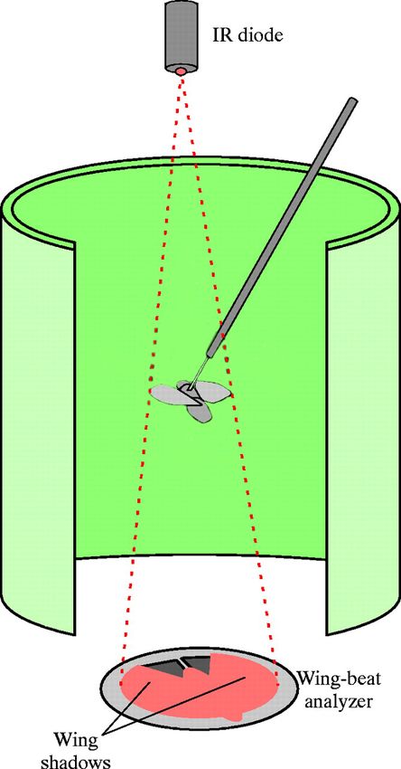
2.2.2 Optical wing-beat analyzer
Wing-beat analyzer equipment (purchased from the James Franck Institute,
University of Chicago, USA) was used to measure characteristics of the wing stroke
during the flight of a tethered Drosophila in real time. The wing-beat frequency and
amplitude of each wing was measured. The difference in the wing-beat amplitudes
of the two wings was used to calculate the fly’s yaw torque (Götz, 1987; Theobald,
Duistermars, Ringach, & Frye, 2008).
Hardware component setup
The wing-beat analyzer consisted of a main circuit unit, a photosensor and an
infrared LED unit (Fig. 1). Each fly was tethered to a tungsten rod and placed
inside the arena such that its pitch angle was 45° from the vertical plane. An
infrared light-emitting diode (IR-LED HSDL-4230, Conrad Electronics,
Schloßstraße 34-36, Berlin, Germany) with an emission peak at 875 nm was placed
above the fly.
The photosensor unit was placed under the fly. It consisted of two infrared-
sensitive silicon wafers, placed so that the shadow of one wing would be recorded by
one sensor and the shadow of the other wing would be recorded by the other sensor.
19 | P a g eEach sensor was connected to an adjustable current amplifier. A crescent-shaped
cutaway mask was positioned above the photosensor (Fig. 2). A wavelength-specific
visible light attenuator (400-700 nm, FWHM 400 nm, Filcom Photomask Inc.
Japan) was kept above this mask to ensure that only the light from the IR LED
reached the sensor.
The relative position of a fly was calibrated by moving the fly holder using a
micromanipulator, such that the shadow caused by the wing fell on the cutaway
mask. The size of the shadow was adjusted by moving the fly and the IR-LED so the
shadow was laterally centered over the cutaway mask (Fig. 2). The mask and
amplifier ensured that the final output was proportional to the position of the
shadow cast by the beating wing. The output voltage represented the shadow of the
wing beat, which increased during the forward excursion of the wing.
The photosensor unit transmitted a current proportional to the shadow of the
wing, which was not blocked by the mask. These analog signals were filtered with a
low pass filter (LPF) with the LPF cut-off set to 1 KHz. The main unit calculated
the frequency and the amplitude of individual wing beats. Finally, the calculated
wing beat amplitudes were routed to the output connectors.
20 | P a g eA
B
Envelope of stroke
amplitude
Sensor
Outline of
mask
Fig. 2. Schematics of the wing-beat analyzer experimental setup.
A. A tethered fly was placed in a hovering position inside the flight arena. Each fly’s
wing stroke amplitude was measured by optically tracking the wing shadows cast
by the infrared LED. Yaw turning was calculated by subtracting the wing-beat
amplitudes of the left and right wings. B. Alignment of the wing shadow (striped
area) over the cutaway mask (grey area). The shadow cast by the wings was
laterally centered over the cutaway mask.
21 | P a g eFig. 3. Typical wing-beat signal obtained from the wing beat analyzer.
Plotted are the two peaks that represent the downstroke and upstroke of an
individual wing during a single wing stroke. The larger peak is followed by a
smaller peak (Source: JFI electronic laboratory, Chicago).
Inputs to wing beat analyzer equipment
The gain level was adjusted to produce 4 V at the final amplitude signal from
the signal-out connectors. Flip excursion was set to 1.5 ms. The gating pulse widths
R2 and R29 were set to 1.2 ms for the left and right channels. A source was selected
from left or right to set the gating level. The low-pass filter (LPF) cut-off was
adjusted to 1 kHz, fine gain to 0.2, coarse gain to 100, trigger lever to 0.40 and gate
width to 9.8. The potentiometer in the sensor was adjusted to a unit gain of 5 out of
11.
2.2.3 Signal optimization
The photocurrents obtained from the sensors were transmitted to the main
unit to calculate the frequency and amplitude of the wing stroke. The end analog
signals corresponding to the calculated yaw torque were converted to computer-
readable digital signals using a sampling frequency of 250 Hz. Converter equipment
with 12-bit successive approximation (ADC-USB-120FS, Measurement Computing
22 | P a g eInc., USA) was purchased for analog-to-digital data conversion. These converted
digital signals were reformulated by employing a moving average filter in MATLAB
software (MATLAB 2011a, version 7.12.0, MathWorks Corporation, USA.). The
following equation was applied to govern the filtering strategy, used with an
averaging factor (M) of 13:
where x = the input signal, y = the output signal and M = the averaging factor.
2.3 Modular Display system
An electronic display system was used to display an unvarying visual
environment in the flight arena. A fly was usually tethered and surrounded by the
cylindrical flight arena. Earlier studies utilized a rotating mechanical cylinder to
display the visual stimulus (Götz, 1968). This original apparatus has recently been
improved by replacing the mechanical components with an electronic controller
system (Reiser & Dickinson, 2008). This display system, combined with wing beat
analyzer equipment, was used for the spontaneous flight behavior studies. A
homogeneously illuminated electronic arena was used in this study. There was only
nonpatterned, uniform green illumination on the arena wall.
Hardware setup
The electronic display system contained a circular array of light-emitting
diodes (LED) panels (BM-10288MI, American Bright Optoelectronics Corp.,
Magnolia Ave, Chino, USA), two panel controller boards (PCB) and a Panel Display
Controller (PDC) (Mettrix Technology Corp., Hopewell Junction, New York, USA).
Each LED module (32 mm × 32 mm × 19 mm) consisted of an 8 X 8 matrix array of
green LEDs with an attached microprocessor unit. The cylindrical arrays of LED
23 | P a g epanels were assembled in 4 X 12 LED panel formations making up a volume of 1448
cm³. This cylindrical unit was positioned between two panel controller boards
(PCB). One of the PCBs was connected to the PDC (Fig. 4). In this specific setup, no
coupling was established between the flight arena and the wing beat analyzer’s left
(L) and right (R) wing beat amplitudes, thereby leaving open the feedback loop
between the fly’s behavior and the panorama.
The angle between adjacent LEDs was 1.7°. The luminescence of the arena
was 72 cd/md², and the contrast level at maximum display was 92%. Each LED was
refreshed at 370 Hz (Reiser & Dickinson, 2008), which is below the flicker fusion
rate of the fly (~200 Hz). The spectral intensity was ~0.4 at an intensity level of –3,
and the wavelength of each LED was ~560 nm. This wavelength has been shown to
drive R1-R6 photoreceptors in Drosophila (Wu & Pak, 1975). The room lights were
turned off during the machine operation. Because this methodology of assembling
the arena and programming the panels and control programs was adapted from a
web resource https://bitbucket.org/mreiser/panels/wiki/Old_Panels_Info, no detailed
steps to program individual LED panels and assemble the arena are provided in
this section.
24 | P a g eFig. 4. Schematics of the LED arena setup. An insect Panel Display Controller (PDC) retrieves display patterns from a memory card (CF) and transmits them to each panel (P) through a TWI connector. A control program in the computer (PC1) connected with the PDC via RS232 offers GUI-based controls to access the display parameters. All units are powered by a 5 V DC power supply unit (PSU1). Overview of working components PC software: We used a MATLAB-based software program for communication with the PDC. This program is accessible via the MATLAB software to generate patterns, control intensity and communicate with the controller boards. The intensity level was set to 3 units to maintain constant illumination. 25 | P a g e
Panel Display Controller (PDC): The panel display controller consists of a dual
microcontroller circuit unit. A flash microcontroller unit (ATmega8, Atmel Corp.,
San Jose, CA, 95110, USA) reads pattern data from the CF card and delivers it to
the main microcontroller unit. The main controller receives the data from the PC
control program over the serial port (RS232) and maintains display updates. It also
communicates with external devices over Analog Input (AI), Analog Output (AO),
and Digital Input/output (DIO) ports.

Computer system (PC1):       Intel Pentium 4 CPU 1.60GHz, 2 GB RAM, NVIDIA
Quadro4 700 XGL, Maxtor 53073H6 75GB HDD, Windows 7.

An Atmel AVR ISP MKII in-system programmer (SKU: ATAVRISP2, Atmel
Corporate Headquarters, 1600 Technology Drive, San Jose, CA 95110, USA.) was
used to program the microcontroller units (MCUs) of the LED panels and the panel
display controller (PDC). This flash programming was done using a soft kit Atmel
AVR studio 4 software package (http://www.atmel.com/tools/avrstudio4.aspx).

A CompactFlash card (CF): Traveler CompactFlash, 64 MB, was used to store the
pattern data.

Panel unit (P): The panels are individual display modules with an 8 X 8 green dot
matrix array of LEDs and a supporting microcontroller unit (MCU) to refresh the
display locally. An MCU receives the pattern data and refreshes the LED display in
every LED panel.

2.4 Analysis of yaw torque data

2.4.1 Fast Fourier Transform (FFT)
       Fast Fourier Transform (FFT) was used to detect the frequency components
of any oscillations arising from the fly behavior or the equipment. The FFT function
in MATLAB transforms the time domain of a discrete time series sequence into a
frequency          domain.              MATLAB          software          functions

26 | P a g e
(http://www.mathworks.de/de/help/matlab/ref/fft.html) were used for these
transformation. These functions utilize the following equation.
The functions Y = fft(x) and y = ifft(X) implement the transform, given for vectors of
length N by
where
is an Nth root of unity (Duhamel P, 1990).
The window length of the raw data was converted to a length (N) to increase the
calculating efficiency for the relatively larger datasets.
2.4.2 S-Map procedure
The S-Map procedure was applied to the yaw torque signals obtained from
the wing beat analyzer equipment. S-Map stands for a sequentially locally
weighted global linear map. The S-Map procedure is a tool that can be used to
quantify the nonlinearity of given time series data by utilizing nonlinear forecasting
analysis. This tool is able to detect a pattern in data that otherwise appear to be
random using sample prediction and the complexity of the dynamic system. The
given dataset is broadly considered to arise from a dynamic system that is bound to
dynamic rules. The dynamic system determines the unique successor stage at any
consecutive time after sampling the first half of state variables. If the system is
linear, the initial conditions can be used to determine the subsequent state of the
linear system. When the system does not follow the linearity equation, the system
tends to deviate from an ideal linearity. In that case, the system can be a nonlinear
dynamic system.
27 | P a g eThe S-Map procedure takes the first half of the points in a time series and
predicts the second half of the data series. The first half of the data points is
embedded to create attractor values, which are then used to predict the second half
of the time series. Embedding is basically plotting time values against past values
of the data. The general idea is that past values can be used to reconstruct the
equation that generated those values. The shape that emerges from this embedding
is called an “attractor”. The second half of a time series of values can be predicted
using this equation. An algorithm selects points that have histories similar to the
initial points and that fall near the predicted values of the attractor. A new
regression is computed for every prediction such that the vectors that are most
similar to the predicted values are weighted more heavily. The points near the
predicted values have more influence on the shape and direction of a line. All (not
just some) of the points chosen are projected, and those points are exponentially
weighted (Maye et al., 2007). If the system is globally linear, the best forecasts use
all of the points in the attractor and not under-represent any of them. The accuracy
of these predictions is evaluated by the coefficient of correlation between the
predicted and the observed series.
However, if the relationship between actual and predicted data is more
complicated, then the models increase the weighting parameter (Φ) to access the
nonlinear status of the system (higher correlation values when Φ > 0). If the
manifold is dominated by noise, it appears as being only weakly nonlinear. So the S-
Map method offers more skillful forecasts.
The function w is used to weight the library vectors by their distance to the
prediction vector:
For Φ = 0, a linear map is obtained. Increasing Φ puts increasingly greater
emphasis on the library vectors close to the prediction vector. MATLAB scripts for
28 | P a g ethe S-Map analysis were obtained from Dr. Alexander Maye, University Medical
Center Hamburg-Eppendorf, Germany.
Fig. 5. A simplified interpretation of the S-Map analysis.
The correlation coefficient of the actual and predicted data against the weighting
parameter is plotted. A shallow curve results if the relationship between the actual
and predicted matrices is globally linear. When this relationship is complicated,
weight is given to the predicted dataset to access the nonlinearity of the system
(Maye et al., 2007). Thus, by increasing the weighting parameter, the steepness of
the curve would indicate the presence of a nonlinear signature.
Quantification of the S-Map procedural results
The steepness of the curve over an increasingly weighted parameter in S-
Map analysis determines the level of nonlinearity. A shallow curve indicates a
globally linear signature in the S-Map procedure (Maye et al., 2007). Thus, the slope
of a least-square regression line is calculated to estimate the nonlinearity of a time
29 | P a g eseries. A first-degree polynomial curve, in a least square sense in MATLAB software
(function: ‘polyfit’), was used to calculate the slope coefficients. The increase in the
slope value denotes the estimated increase of a nonlinear signature.
2.4.3 Spike detection algorithm
Torque spikes were detected by applying spike detection algorithms. The
spike detection algorithms written in the MATLAB software were adapted from
Maye et al., 2007.
Raw yaw torque data were first filtered by a direct form II transposed
implementation of the standard difference equation. Maximal and minimal values
were detected from the filtered matrices by shifting the filtered values step-by-step
in an array according to the user-defined threshold and step length. These
maximum and minimum values were sorted out as spikes over the defined step
length. The variables closest to a sorted variable were ignored using defined step
lengths. Amplitude threshold levels were set from -1 to 1, depending on the filtered
signal’s amplitude. A detection frequency of 150 Hz was used.
2.4.4 Geometric Random Inner Product (GRIP) analysis
A GRIP analysis was implemented on the intervals between each torque
spike. The GRIP procedure, developed by Maye et al., 2007, was used in this study
to quantify the deviation from theoretically expected ideal randomness.
Randomness is defined in terms of radioactive decay (Krane, 1988), whereas non-
randomness was quantified by excess repetitions (i.e., repeats) or alternations
between the successive bits (i.e., switches). The GRIP analysis assumes that a given
vector represents a randomly distributed sequence. The average inner product of
randomly distributed vectors in n-dimensional geometric objects is aggregated
according to object-specific constants. The deviation from these constants was used
as a measure of the randomness of a given dataset. This method is applied to the
inter-saccade intervals (ISI) and inter-activity interval datasets with the Buridan
paradigm to assess the randomness of the inter-event interval distribution.
30 | P a g e2.5 The Buridan Paradigm
2.5.1 Flies
Experimental flies (mixed sex unless otherwise stated) 2-3 days old were
anesthetized by briefly exposing them to carbon dioxide gas. One-third of a wing
was left intact and rest was clipped using a pair of fine scissors. Wing-clipped flies
were kept overnight in small containers with sugar granules and moistened tissue
paper.
In brief, the Buridan paradigm (Colomb et al., 2012) device was used for
automatic tracking of a walking fly given free choice between two visual landmarks
in order to assess general locomotor competence. General characteristics of walking
flies such as duration of walking, speed, etc. was calculated from this paradigm.
2.5.2 Hardware components
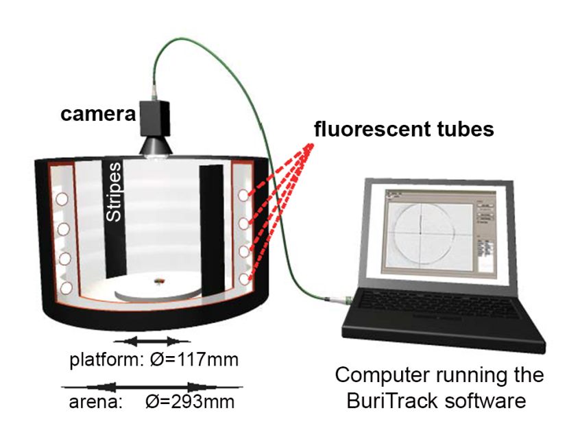
The Buridan paradigm consists of three components: a cylindrical arena, a
standard USB camera (Logitech Quickcam Pro 9000) and a computer system.
The cylindrical unit consists of a round platform measuring 117mm in
diameter. The cylinder was illuminated by four circular fluorescent tubes
surrounding it (Osram, L 40w, 640C circular cool white).The four fluorescent tubes
are located outside the cylindrical diffuser positioned at a distance of 147.5 mm
from the center of the arena. Alternating current (1 kHz) was provided to the tubes
by an electronic control gear (Osram Quicktronic QT-M 1×26–42). The inner area of
the cylinder was outfitted with two opposing horizontal stripes inaccessible to the
flies. The stripes were taped to the inside of the diffuser and each stripe measures
30mm X 313mm X 1mm. A standard USB camera was placed above the arena as
depicted in Fig. 5 and the camera is connected to the computer running tracking
programs. A wing-clipped fly was placed in a center of the platform during an
experiment. The temperature on the platform during the experiment was 27°C, and
31 | P a g ethe luminosity ranged from 7.5 to 8 klx, with light intensity ranging from 370 to 850
nm.
Fig. 6. Picture of the Buridan paradigm setup:
A wing-clipped fly was placed in the middle of a platform (117 mm diameter). The
cylindrical arena surrounding the platform was constantly illuminated by
fluorescent tubes. This arena was furnished with two horizontal black stripes
measuring 30 mm wide, 313 mm high and 1 mm thick. A water canal between the
arena and platform prevents the fly from reaching the stripes. The fly’s position is
captured on video using the standard USB webcam and transmitted to the tracking
algorithm for extracting fly trajectory coordinates. (Cartoon Source Colomb et al.,
2012).
2.5.3 Tracking software BuriTrack
An open source Buridan paradigm software package containing the tracking
programs and analysis scripts were downloaded from http://buridan.sourceforge.net/
and installed on the computer. BuriTrack is a tracking program that captures the
darkest spot in a given pixel range determined by a user threshold. This spot is
taken as the assumed position of the fly. The tracking program stops and records a
burst event whenever the fly jumps outside of the platform boundary. The final
32 | P a g etrajectory data (X, Y in pixels), the time stamp and burst counts were saved as a
text file (ASCII). The total duration of the experiment was set to 20 min. The
graphical user interface offers the flexibility of choosing the threshold and other
tracking factors.
2.5.4 CeTrAn Centroid Trajectories Analysis software
The dataset generated by a BuriTrack algorithm was analyzed using a
CeTrAn trajectory analysis algorithm written in open source statistics package R
(http://r-project.org/). The graphical user interface given in the package (Colomb et
al., 2012) was utilized to import the trajectory dataset. The median speed, meander,
and activity parameters were computed using the analysis program.
2.5.5 General activity measurement
Activity and median speed
The algorithm considers every movement an activity and every absence of movement
longer than 1 s is taken as a pause (shorter periods of rest were considered active periods).
Activity was calculated in seconds. Speed was calculated by dividing the distance over instant
speed of each movement of a fly (mm/s). The mean of the median speed of each fly was
calculated to measure the speed performance of the group. Speed value exceeding 50 mm/s was
considered a jump and was not included in the calculation.
Computer-generated walking data
The computer-generated data was obtained from the following web source:
http://buridan.sourceforge.net/. These data samples were generated by modifying
the R code from an adehabitat package. The direction was set to follow a correlated
walk. An initial angle was chosen randomly and the next one was generated
following a wrapped normal distribution around the previous angle. The correlation
strength between two consecutive turning angles was determined by a variable ‘r’. A
step length for the 8999 movements (900 seconds at 10 Hz) was created by
multiplying a Boolean variable simulating pauses (1 or 0, randomly generated using
a uniform distribution with adjustable frequency “f”) with a speed value that was
33 | P a g ecreated by drawing from a Chi distribution around a mean value “h” (correlated
walk) (Colomb et al., 2012).
The position was calculated iteratively, starting at the center of the arena.
When the position fell outside the boundary, it was replaced by the nearest point
within the limits of the arena and the angle sequence was recalculated taking the
first angle randomly. Accordingly, the next movement will lie outside of the
platform with a probability >0.5.
2.5.6 Inter-activity interval extraction
Activity intervals were extracted from Buridan activity datasets. The time
interval between each start of activity was considered an inter-activity interval. In
Buridan’s paradigm, every movement is considered an activity and every absence of
movement longer than 1s is a pause (shorter periods of rest were considered active
periods). These inter-activity intervals were tested for randomness using GRIP
analysis.
2.6 pySolo assay
2.6.1 Flies
Experimental flies 2-3 days old were kept overnight in small fly containers
with a few sugar granules and moistened paper. The next day, the flies were loaded
into a pySolo chamber for experimentation.
pySolo is a python-based tracking program designed for drosophila sleep and
locomotor pattern analysis (Gilestro, 2012). pySolo was used to measure the
locomotor activity performance of the Drosophila. All tracker programs, analysis
scripts and detailed instructions on setup and usage were obtained from a web
resource www.pysolo.net.
34 | P a g e2.6.2 Hardware components
The setup consists of 12 test tubes, each measuring 70mm X 3mm, a
cardboard box, low voltage infrared light emitting (IR-LED) diode stripes (BLO106-
15-29, Conrad electronics, Germany), a USB camera (Logitech Quickcam Pro 9000)
and a computer.
Each tube was sealed with food on one side and a cotton stopper on the other.
These tubes were placed together a few millimeters apart inside the box and closed
with a transparent sheet. Infrared red light emitting diode stripes were placed
above these tubes to illuminate the setup without any reflective glare. The camera
was placed above this box, in such a way that the individual test tubes were visible
in the pySolo video monitor. The IR filter was removed from the USB camera to
capture the infrared illumination (Fig.7).
2.6.3 Configuration
pySolo tracking software was installed on the computer with an Ubuntu
operating system (10.04.4 LTS-Lucid Lynx) as per the instructions given in the web
tutorials from www.pysolo.net. Once installed on the computer, pySolo is accessed
through the command line by typing the following command:
pysolo_anal.py -c alternative_options.opt
This will start a program along with an optional file for editing any user
preferences. An intuitive graphical user interface offers the flexibility of editing
preferences. The following parameters were set to record from a single camera
monitoring system.
The essential data to be filled in are in the first window, under ‘Files and Folder’.
They are
• the DAM folder
• the output folder
35 | P a g eYou can also read