Trajectory Optimization for Manipulation of Deformable Objects: Assembly of Belt Drive Units
←
→
Page content transcription
If your browser does not render page correctly, please read the page content below
Trajectory Optimization for Manipulation of Deformable Objects:
                                                               Assembly of Belt Drive Units
                                                   Shiyu Jin1 , Diego Romeres2 , Arvind Ragunathan2 , Devesh K. Jha2 and Masayoshi Tomizuka1
                                                                 1 University   of California, Berkeley, 2 Mitsubishi Electric Research Laboratories
                                                              1 @berkeley.edu, 2 @merl.com

                                            Abstract— This paper presents a novel trajectory optimiza-                           6 DOF robot                    Pulleys
                                         tion formulation to solve the robotic assembly of the belt
arXiv:2106.00898v2 [cs.RO] 21 Jun 2021

                                         drive unit. Robotic manipulations involving contacts and de-
                                         formable objects are challenging in both dynamic modeling
                                         and trajectory planning. For modeling, variations in the belt
                                         tension and contact forces between the belt and the pulley
                                         could dramatically change the system dynamics. For trajectory
                                         planning, it is computationally expensive to plan trajectories for     F/T sensor                              P2
                                         such hybrid dynamical systems as it usually requires planning                                                                        P1
                                         for discrete modes separately. In this work, we formulate the          Parallel jaw gripper
                                         belt drive unit assembly task as a trajectory optimization
                                         problem with complementarity constraints to avoid explicitly                                 Belt
                                         imposing contact mode sequences. The problem is solved as
                                         a mathematical program with complementarity constraints
                                                                                                              Fig. 1. Belt drive unit assembly task. The robot grips a polyurethane belt
                                         (MPCC) to obtain feasible and efficient assembly trajectories.       and assembles it on two pulleys, P1 and P2 .
                                         We validate the proposed method both in simulations with a
                                         physics engine and in real-world experiments with a robotic
                                         manipulator.
                                                                                                              aims to design a finite-time input trajectory, u(t), ∀t ∈ [0, T ],
                                                               I. I NTRODUCTION                               which minimizes some cost functions over the resulting
                                            While we have seen tremendous developments in the fields          input and state trajectories [13]–[15]. In the belt drive unit
                                         of artificial intelligence in recent years [1]–[4], robots can       assembly, variations in the belt tensions and contact forces
                                         achieve only limited autonomy during manipulation tasks [5].         between the belt and the pulleys result in a hybrid dynamical
                                         One of the biggest challenges that restricts general-purpose         system. Elastic force can exist or not, depending on whether
                                         manipulation algorithms is contact dynamics. Contact-rich            the belt is slack or stretched. Contact forces can exist or
                                         manipulation tasks are difficult to solve from both modeling         not, depending on whether the belt contacts the pulley or
                                         and optimization perspectives. The manipulation problems             not. Both elastic and contact forces might greatly impact the
                                         become further challenging when the manipulated objects              system dynamics. Planning for such a hybrid system usually
                                         are deformable. These kinds of objects are ubiquitous in             requires planning for each dynamic system separately. There
                                         a lot of assembly problems, and yet they remain poorly               are many existing works on trajectory planning for hybrid
                                         understood. In the assembly challenge competition in World           systems [16]–[18]. But the drawback is that those methods
                                         Robot Summit 20181 , assembly of a polyurethane belt onto            require a task-specific mode schedule, which may bring
                                         pulleys (see Figure 1) was one of the most challenging tasks         extensive efforts in modeling and parameter tuning.
                                         [6]. While there have been attempts to solve manipulation               Inspired by the work on trajectory optimization of rigid
                                         problems involving deformable objects [7]–[12], there is no          bodies through contact [13, 15, 19, 20], we model the physics
                                         general approach to it.                                              of contacts and the elastic properties through complemen-
                                            In this paper, we consider the problem of wrapping a              tarity constraints. The elastic belt is modeled through a 3D
                                         belt around a two pulleys system, considering as use case            keypoint representation. The hybrid behavior of the keypoints
                                         the challenge introduced in the World Robot Summit 2018.             is captured by the complementarity constraints. We formu-
                                         Working with a deformable object like the belt presents              late the trajectory optimization problem as a Mathematical
                                         several challenges. These include: (i) infinite degrees of           Program with Complementarity Constraints (MPCC) [21].
                                         freedom for the belt; (ii) contact rich manipulation; and (iii)      We successfully solve the MPCC to compute feasible and
                                         long-horizon planning problem.                                       efficient trajectories to assemble the belt drive unit. Finally,
                                            Optimization-based planning and control may be applied            we implement the solution into the real system with a
                                         to various problems in robotic manipulation. Given a con-            controller to track the optimized trajectory.
                                         trolled dynamical system, ẋ = f (x, u), trajectory optimization        The main contributions presented in this work are:
                                                                                                                 1) Trajectory optimization formulation for deformable ob-
                                           1 https://worldrobotsummit.org/en/about/                                  jects manipulation with complementarity constraints.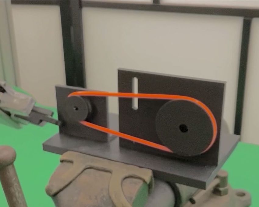
This provides a general-purpose, mathematical frame-
     work to tackle these problems.                                                                               K1
  2) Introduction of 3D keypoint representation for de-
     formable objects.
  3) Validation of the proposed approach through simula-
     tion as well as real experiments.                                                                      L
                     II. R ELATED W ORK                                                Yaw
                                                                                             Z
   Deformable linear (one-dimensional) object manipulation                            Y              Roll         K2
                                                                                                 X
has been studied for decades. A randomized algorithm was                           Pitch
proposed to plan a collision-free path for elastic objects
[22]. Minimal-energy curves were applied to plan paths for          Fig. 2. Initial belt configuration, ρ0 , with keypoints representation. The
                                                                    red dots represent the “grasped” keypoint K1 and “opposite” keypoint K2 .
deformable linear objects in stable configurations [23]. In         The yellow dashed line shows the virtual cable, C , of length L.
[24], a local deformation model approximation method was
proposed to control the soft objects to desired shapes. The
authors of [25, 26] extended the local deformation model            common assumption in mechanics. The pulleys have known
to the manipulation of cables. A deep neural network was            geometries and can rotate freely around the shafts axis. The
trained to manipulate a rope to target shape based on a             base of the belt drive unit is fixed to the workbench in a
sequence of images [27]. However, those works do not                known pose. We assume that at the initial configuration,
consider the interaction between the deformable cables and          called ρ0 , the belt is grasped and lifted by a gripper held by
the environment. In [7], the authors proposed a strategy to         a robotic manipulator, and the belt is freely hanging under
assemble a flexible beam into a rigid hole. An optimization-        the effect of gravity, see Figure 2. The task objective is to
based trajectory planning was utilized to assembly ring-            wrap the belt around the two pulleys as shown in Figure 1.
shaped elastic objects in [8], but the authors only validated          Inspired by recent work [32], we introduce a 3D keypoints
their method in simulation. In [9], the authors took the            representation for deformable objects. This representation
advantage of environmental contacts to shape deformable             consists of identifying points in the object that are represen-
linear objects by a vision-based contact detector. The authors      tative of the whole object. With the proposed representation,
of [10] considered a scenario to assemble the roller chain          the problem is mathematically tractable with a finite, low
to sprockets. Their strategy successfully assemble the chain        dimensional state space and interpretable constraints and cost
but lacks in generalization because each step is engineered         function. In particular, we select two 3D keypoints for the
for the specific system. To advance the research on robotic         belt as shown in Figure 2. The “grasped” keypoint, K1 ,
manipulation, the World Robot Summit 2018 proposed a                corresponds to the point-mass on the belt grasped by the
competition on assembly challenges [6]. The challenge high-         robot gripper, and the “opposite” keypoint, K2 , which is the
lighted the complexity of solving manipulation tasks in a           point on the belt that is the furthest away from K1 when
general manner, which still remains an open problem.                the belt is in configuration ρ0 . In the proposed keypoint
   Optimization-based methods have been successfully im-            representation, configuration ρ0 can be represented by a
plemented in many trajectory planning scenarios [28]–[30].          virtual elastic cable, C , that connects K1 and K2 . The gener-
[13] proposed a trajectory optimization method for rigid            alized coordinates of the system can now be described as
bodies contacting the environment. They formulated an               q = [K1x , K1y , K1z , K2x , K2y , K2z , K1roll , K1pitch , K1yaw ]> ∈ R9 , where
MPCC to eliminate the prior mode ordering in discontinuous          K1x , K1y , K1z , K2x , K2y , K2z are the Cartesian coordinates of two
dynamics due to inelastic impacts and Coulomb friction. The         keypoints and K1roll , K1pitch , K1yaw are the orientation of K1 with
MPCC framework was extended to a quadrotor with a cable-            reference frame shown in Figure 2. We utilize the orientation
suspended payload system in [31]. The complementarity               of K1 to express the rotation and the twist of the belt. The
constraint was utilized to model the limitation of a non-           action space u = [Fx , Fy , Fz , Mx , My , Mz ]> ∈ R6 is the vector of
stretchable cable length. Inspired by [13, 15, 19, 20, 31],         forces and torques that are applied to K1 through the gripper.
we introduce complementarity constraints to the belt drive          This makes the belt drive unit an underactuated system as
unit assembly task to avoid the hybrid modes selection due          we cannot directly control K2 . Finally, we assume that in
to elastic force in the belt and contact force between the          configuration ρ0 the ellipsoidal shape of the belt is large
belt and the pulleys. We extend the keypoints representation        enough to go around the first pulley P1 .
introduced for rigid objects, [32], to model elastic objects like
the belt and to formulate an MPCC to perform the assembly.          A. Subtasks Decomposition
                                                                       Belt drive unit assembly is a complex task that requires
               III. P ROBLEM F ORMULATION                           a long-horizon planner. As often proposed in the literature,
  The belt drive unit consists of two pulleys attached to           long-horizon planning tasks are decomposed into subtasks
a base and of a deformable and stretchable belt as shown            to reduce complexity. The belt drive unit assembly can have
in Figure 1. The belt is assumed to be composed of a                highly engineered solutions with a dense sequence of sub-
homogeneous isotropic linear elastic material which is a            tasks and simple planners whose subgoals are trivial to reach.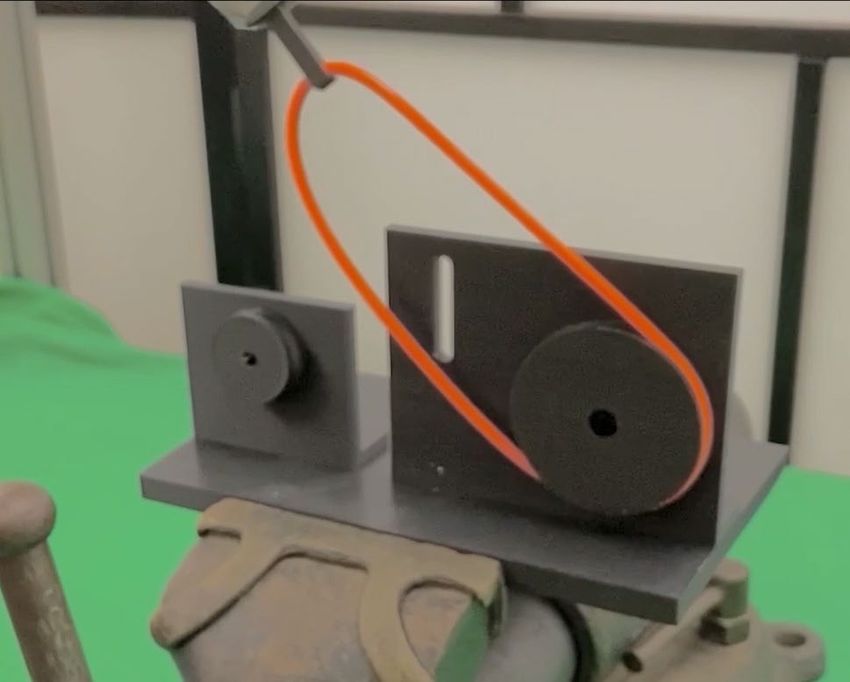
K1 u
Fu K1
g
Fk
λ0
P2 P1 P2 P1 K2 λ1
K2 K1 λ0
g
S1 S2 K2
g
λ1
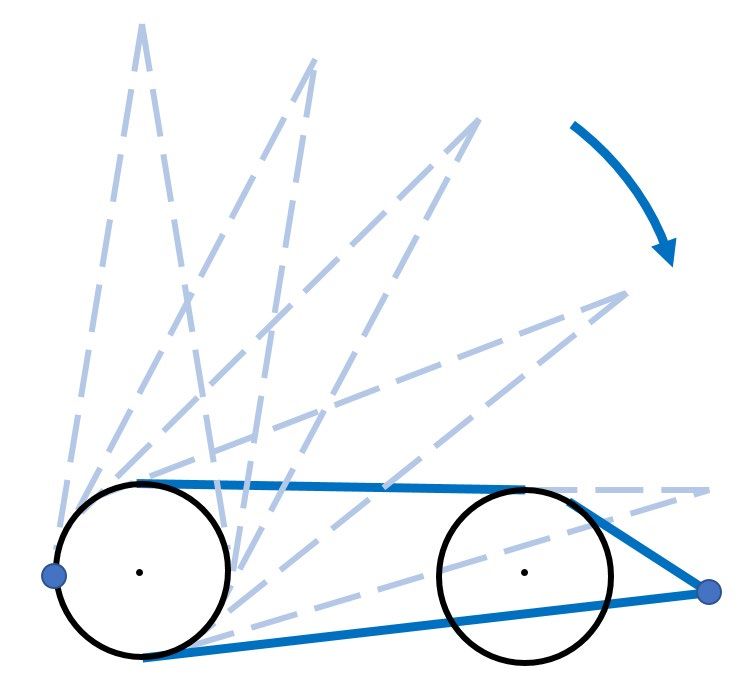
Fig. 3. Two subtasks decomposition. P1 and P2 are two pulleys. The blue
lines represent the belt gripped at keypoint K1 by a robot. S1 : The belt
wraps the first pulley P1 and it stretched. S2 : The belt rotates around the
first pulley and is assembled onto the second pulley P2 . Fig. 4. Force analysis at the two keypoints. Fu is the control input force.
λ0 is the elastic force. λ1 is the contact normal force. g is the gravity force.
However, this kind of approach requires extensive effort in
parameter tuning and engineering work and lacks generality, where L(q, q̇, u, λ ) is the cost function, q ∈ R9 are the gen-
since the goals of the subtasks need to be redefined as eralized coordinates described in Sec. III, q̇ and q̈ are its first
the scenario changes. We partially address this problem and second order time derivatives, u ∈ R6 is the control input
by reducing the number of subtasks to two. Following a and λ are the external forces acting on the belt. Eq. (1b) is the
logic similar to a human’s approach, the first subtask, S1 , forward dynamics, where H(q),C(q, q̇), G(q) are the inertial
corresponds to wrap the belt around the first pulley, and the matrix, the Coriolis terms, and the gravitational forces,
second subtask, S2 , corresponds to wrap the second pulley respectively. B(q) is input mapping. The general nonlinear
keeping the belt taut to maintain the wrap around the first constraints (1c) include the complementarity constraints and
pulley, see Figure 3. In a qualitative description, in S1 , the collision avoidance. Eq. (1d) represents the lower and upper
belt has to avoid the outer surface of the first pulley P1 and K2 bounds of the optimization variables.
has to get into the groove creating a contact force, while K1 We solve (1) as a nonlinear program and use a direct
is stretched until the belt is taut. In S2 , the belt is assembled approach which in general has better numerical properties
on the second pulley P2 by rotation around the first pulley. than shooting methods, and we can exploit the sparsity
During the rotation, the belt should remain taut in order to structure of the problem. We directly optimize the feasible
remain in the groove of the first pulley. Finally, the belt has general coordinates and its first-time derivative, the control
to hook the internal groove of P2 and K1 has to reach the inputs, and the external forces. The discretization of the
bottom of the second pulley to accomplish the task. forward dynamics is obtained by the trapezoidal rule. The
formulation of the contact and elastic forces as complemen-
Given the proposed 3D keypoint representation of the
tarity constraints fits naturally well in this formulation. In
belt drive unit, we can formulate a trajectory optimization
practice, for numerical advantages, we use a relaxed version
problem, that uses complementarity constraints to model the
of the complementarity constraints as described in [33].
contacts and the deformation of the belt, to solve each of
In the following, the dynamical constraints and the cost
the two subtasks. The two optimized trajectories are then
function for MPCC (1) are described for the two subtasks.
executed sequentially in order to accomplish the task, the
final condition of S1 corresponds to the initial condition of S2 . A. Dynamics Constraints
The system is composed of the two keypoints, K1 and
IV. T RAJECTORY O PTIMIZATION FOR THE B ELT D RIVE K2 , and the virtual elastic cable, C . It is modeled similarly
U NIT A SSEMBLY to a mechanical mass-spring-damper second-order system,
We approach the belt drive unit assembly as a trajectory with an actuator acting on K1 and subject to the gravity
optimization problem formulated as an MPCC. The com- and the external forces given by the elastic force λ0 and the
plexity of this problem is given by the presence of hybrid normal force λ1 experienced during contacts. Figure 4 shows
nonlinear dynamics due to contacts that may happen between a schematic example of the forces that act on the system at
the pulleys and the belt, the elastic properties of the belt, the end of subtask S1 . The system dynamics are defined as
the obstacle avoidance constraints, and the long planning ẋ = Ax + Bu + G + f (x, λ ) (2)
horizon. A trajectory optimization problem is solved for each
of the two subtasks described in Sec. III-A of the form where x = [q> , q̇> ]> ∈ R18 is the system state and λ =
[λ0> , λ1> ]> is the vector of the external forces. The state
min L(q, q̇, u, λ ) (1a) transition matrix
q,q̇,u,λ
09×9 I9×9
s.t. H(q)q̈ +C(q, q̇) + G(q) = B(q)u + λ (1b) kd kd
3×9 − m1 I3×3 m1 I3×3 03×3
0
g(q, q̇, u, λ ) ≤ 0 (1c) A= ∈ R18×18
03×9 mkd I3×3 − mkd I3×3 03×3
2 2
q ≤ q ≤ q, q̇ ≤ q̇ ≤ q̇, u ≤ u ≤ u, λ ≤ λ ≤ λ (1d) 03×9 03×9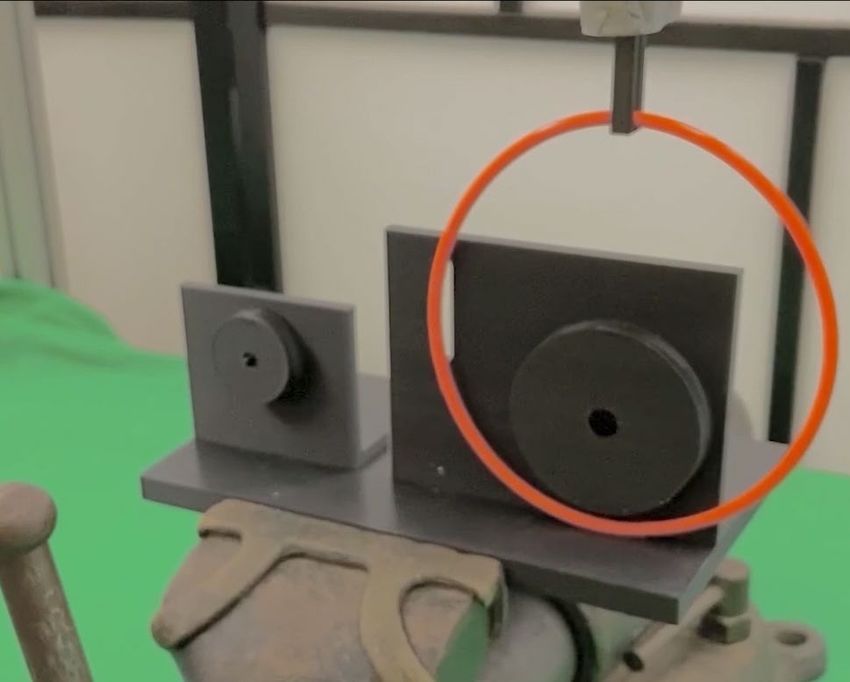
represents the effect of the mass-spring-damper system with λ2 is an algebraic variable. If the cable is stretched, then
kd the damping coefficient and m1 , m2 are the masses of the L < l(x), λ̄0 > 0, and λ2 = 0. If the cable is slack, then
keypoints K1 and K2 , respectively. The input matrix L > l(x), λ̄0 = 0, and λ2 > 0.
Contact force constraint. The second complementarity
09×6
I3×3 0 constraint is formulated as
3×3
B = m1 ∈ R18×6
q
03×6 λ3 = ||K2 − Oe ||2 + ε 2 ≥ ε (5a)
I3×3
03×3 M 1 λ̄1 ≥ 0 (5b)
maps the 6-dimensional end-effector force/torque input u to λ̄1 λ3 = 0 (5c)
the linear and angular acceleration of the “grasped” keypoint
K1 . M1 is the moment of inertia of K1 . The gravitational where Oe is the contact point on the edge of P1 . ε denotes a
acceleration is applied to the two keypoints through the small number to relax the complementarity constraint [33].
> λ3 is the algebraic variable describes whether the belt con-
vector G = 01×11 , −g, 01×2 , −g, 01×3 ∈ R18×1 .
The contribution of the external forces is now given by tacts the pulley. If the belt contacts the pulley, then λ3 = ε,
the sum of the elastic and normal force f (x, λ ) = λ0 + λ1 . and contact force λ̄1 ≥ 0. If there is no contact, then λ3 > ε,
The elastic force is defined as and contact force λ̄1 = 0.
h i>
I I3×3 C. Obstacle avoidance
λ0 = 03×9 , − 3×3
m1 , m2 , 03×3 ΠK1 ,p λ̄0 ∈ R18×1
This constraint imposes that the keypoints cannot pen-
where λ̄0 ∈ R is the magnitude of the elastic force and is etrate into the pulleys. Each pulley is approximated
y
[(K x −px ),(K1 −py ),(K1z −pz )]>
the variable optimized, ΠK1 ,p = 1 ||K1 −p|| is with an ellipsoid, since there is a known analytical ex-
the projection operator of the elastic force into the 3 axis. pression of the distance function between a point and
The point p is K2 in S1 and O1 in S2 for simplicity of an ellipsoid. The obstacle avoidance constraints between
computation. O1 is the position of the first pulley’s center. a keypoint Ki and q a pulley Pj can be denoted as
The normal force due to the contacts between the pulley and distance(Ki , Pj ) = (Ki − O j )> S(Ki − O j ) − 1 ≥ 0, where
the keypoint K2 is defined as
S = diag{1/a2 , 1/b2 , 1/c2 } is a diagonal matrix, a, b, c are
i>
half the length of the principal axes. O j denotes the center
h
I
λ1 = 03×12 , − 3×3
m2 , 03×3 ΠO1 ,K2 λ̄1 ∈ R18×1
of pulley Pj .
where λ̄1 ∈ R is the magnitude of the normal force and is the
y y
[(ox −K x ),(o −K ),(oz −K z )]> D. Physics Limitation
variable optimized and ΠO1 ,K2 = 1 2 ||o1 −K2 || 1 2 is
1 2 The belt might break if stretched over a certain limit, this
the projection operator of the normal force into the 3-axis.
condition is approximated by constraining the length of the
B. Complementarity Constraints virtual cable C , l(x) ≤ Lmax . Moreover, Lmax is assumed large
In order to model the hybrid dynamics due to elastic force enough for the loop to go around two pulleys.
and contact force, we use complementarity constraints
E. Cost Function
0 ≤ g(·) ⊥ h(·) ≥ 0 (3) We use a common quadratic cost function that penalizes
Complementary constraints are a way to model constraints the difference to the goal state xgoal and the control in-
that are combinatorial in nature and impose the positivity put u(k):
and orthogonality of the variables. N
Elastic force constraint. The first complementarity con- J(x, u, λ ) = ∑ (x(k) − xgoal )> Q(x(k) − xgoal )+ (6)
straint is formulated as k=0
T
u(k) Ru(k) + w(λ̄0 (k) − λ̄0desired )2
λ̄0
λ2 = + L − l(x) ≥ 0 (4a)
kp where the weights Q and R are diagonal matrices and w is
λ̄0 ≥ 0 (4b) a scalar. Moreover, the term w(λ̄0 (k) − λ̄0desired )2 adds a soft
constraint in the elastic force. A positive λ̄0desired encourages
λ̄0 λ2 = 0 (4c) a solution with the belt in tension. This constraint is used
where L and k p are respectively the length at configuration in subtask S2 to maintain the belt taut. Instead, in S1 we set
ρ0 and the stiffness coefficient of the virtual elastic cable, C . w = 0.
The length of C at each temporal instant is l(x) = ||K1 − K2 ||
in S1 , and l(x) = ||K1 − O1 || + r1 in S2 , where r1 denotes the V. E XPERIMENTAL R ESULTS
radius of P1 . The pulley center O1 is chosen because it is a In this section, we present the results of the proposed
fixed known point while the pulley is rotating. From eq. (4a) method both in simulation using the physic engine Mu-
the elasticity of the belt is defined as proportional to the JoCo [34] and in a real system with a 6-DoF manipulator.
length L − l(x) and depends on the stiffness coefficient k p . We use the Ipopt [35] solver in a python wrapper.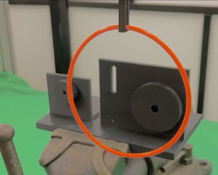
0.1
A. Simulations
X (m)
0
1) Simulation Setup: The belt drive unit is represented
-0.1
in a simulated environment in MuJoCo as shown in the 0 1 2 3 4 5 6
top left corner of Fig. 5. The environment includes two Time (s)
pulleys and one belt. The radius of the pulleys are of 30[mm] 0.7
for P1 and 15[mm] for P2 . The belt is composed of 41
Y (m)
linked objects called capsules in MuJoCo. Any two adjacent 0.6
capsules are connected by two hinge joints and one prismatic
0 1 2 3 4 5 6
joint. The physical properties of the simulated belt are tuned Time (s)
to resemble the belt of the real belt drive unit. The belt is
held by a parallel gripper attached to a 6 DOF Fanuc LR-
Z (m)
0.4
Mate 200iD. The purpose of the manipulator is to actuate
the end-effector in order to track the optimal trajectory, but 0.2
0 1 2 3 4 5 6
in simulation could be removed. Time (s)
Fig. 6. Trajectory of keypoint K1 in a successful assembly for scenario
Figure 5(3). The dashed line is the reference trajectory obtained from
MPCC. The solid line is the measured trajectory.
the belt and the environment and the deformation of the belt
for reaching the desired target.
In the second subtask S2 , the goal, qgoal 2 , is set only for
(1) (2) K1 in both the Cartesian coordinates and angular orientation,
according to the position of the pulley, P2 . A qualitative
representation of the goal position is shown in Figure 5 for
each of the scenarios. The desired [K1roll , K1pitch , K1yaw ]> is
[−π/2, 0, π/2]> . The twist of the virtual cable C approxi-
mates the twist of the belt which leads to the assemble onto
the groove of the pulley P2 . Based on qgoal 2 and k p it is
possible to compute the target elastic force as λ̄0desired , which
encourages the belt to be stretched during rotation.
We perform 10 experiments for each scenario. In each
(3) (4) experiment, the goal positions of the “grasped” keypoint K1
are sampled from the normal distributions N (µ1 , Σ) in S1
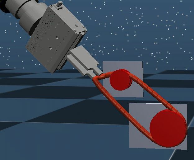
Fig. 5. Snapshots of 4 different simulation scenarios at the goal position of and N (µ2 , Σ) in S2 . Where, µ1 , µ2 ∈ R3 are the components
subtask S2 . The relative positions of the two pulleys vary in each scenario.
[K1x , K1y , K1z ]> in a pre-selected successful qgoal1 and qgoal
2
and Σ = diag{0.005, 0.005, 0.005}. The lower and upper
2) Trajectory Optimization in Different Scenarios: In or- constraints of position, velocity, tilt angle, and force are
der to verify the generality of the approach to different known ±1m, ±0.5m/s, ±π, and ±50N, respectively.
geometries, we consider 4 different scenarios, where the 3) Results: The simulation results are shown in Table I.
position of P1 is fixed and the position of the smaller pulley We initialize the trajectory with all states x(k) = x(0), where
P2 varies, see Figure 5 and Table I. Each pulley is modeled k = 0, 1, .., N. The solver finds a feasible trajectory for both
as three adjacent cylinders, and the two outer cylinders have subtasks given any sampled goals. The optimal trajectory
larger radius than the inner one. The belts’ lengths, Pbelt , are obtained for K1 is then tracked by the end-effector, and the
chosen in each scenario based on the distance between two assembly is completed successfully in 34/40 experiments.
pulleys. The mass of the keypoints is m1 = m2 = 0.042[kg]. The failure cases happen when the goal is sampled away
The moment of inertia of K1 is M1 = 10−7 [kgm2 ]. The belt’s from qgoal1 or qgoal
2 because the belt fails to wrap around the
stiffness and damping coefficient are k p = 63.34[N/m] and pulley. The purpose of these experiments is to show that the
kd = 4.65[Ns/m], respectively. engineering effort in finding the goal position for the subtask
In the trajectory optimization formulation described in is reduced as it is not required to provide one specific point.
Section IV, the goal for subtask S1 is set vertically But also the trade-off of having only two keypoints, more
above the pulley P1 for keypoint K1 , and right un- keypoints would make a more accurate model but also a more
der the pulley P1 for keypoint K2 , respectively, e.g., complex optimization problem. We use an Intel 12 Cores i7-
qgoal
1 = [0.10, 0.55, 0.53, 0.10, 0.23, 0.34, 0, 0, 0]T and both 9850H CPU @ 2.60GHz. The average computational time
with zero velocity. In this substask there is a change of for one trajectory with 600 time steps is 36.138 ± 5.747[s].
mode in the dynamics from no contact to contact between The computational time highly depends on the number of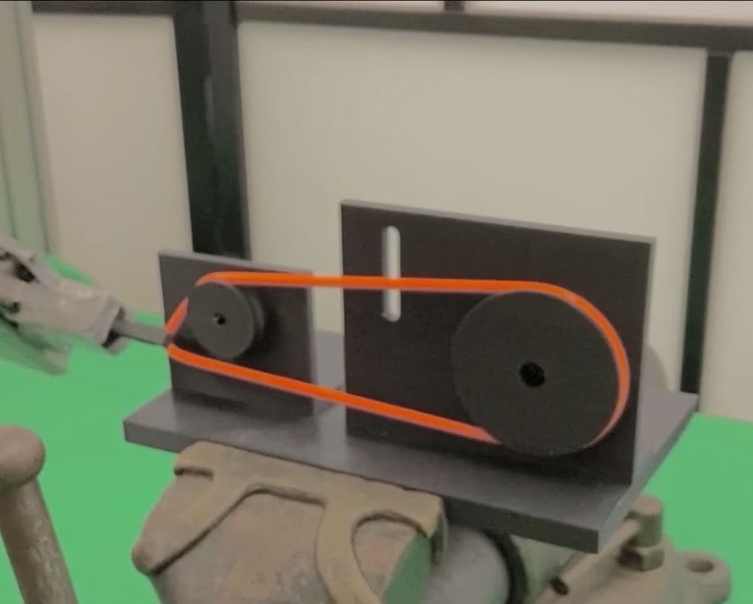
TABLE I
S IMULATION RESULTS IN 4 SCENARIOS . I N EACH SCENARIO THE POSITION OF THE PULLEY CENTER O2 VARIES .
Pbelt O1 (center of P1 ) O2 (center of P2 ) Feasible trajectory Successful assembly
Scenario 1 0.4m [0.100, 0.550, 0.340] [0.100, 0.680, 0.340] 10/10 10/10
Scenario 2 0.4m [0.100, 0.550, 0.340] [0.100, 0.642, 0.432] 10/10 8/10
Scenario 3 0.4m [0.100, 0.550, 0.340] [0.100, 0.645, 0.275] 10/10 7/10
Scenario 4 0.6m [0.100, 0.550, 0.340] [0.100, 0.780, 0.340] 10/10 9/10
trajectory. In the beginning, (Figure 7a), the belt approaches
the pulley and position X increases and the forces are zero.
Z The position Z goes down at 5.57[s] to avoid the outer
Y X
cylinder of the first pulley. At 6.29[s], position X stops
increasing because the pulley is reached (Figure 7b). Then
(a) (b) (c)
the Z position increases as the belt is lifted and contacts the
pulley at 7.82[s] with a corresponding increase in force along
the negative direction in Z. At 10.50[s], the system accom-
plishes S1 (Figure 7c). After that, the belt is rotated around
O1 (the Z position decreases, and Y position increases) while
(f) (e) (d) being stretched (Figure 7d). In this phase, the measured net
force is closed to the desired elastic force λ̄0desired . The target
Fig. 7. Snapshots of the experiment. orientations are [K1roll , K1pitch , K1yaw ]> = [−π/2, 0, π/4]> . The
belt is twisted so that it hooks the second pulley without
Forces vs Time jamming. Finally, the goal of subtask S2 is reached at 29.00[s]
20
(Figure 7e) and the gripper releases the belt (Figure 7f).
Forces (N)
0
The experiment has been repeated multiple times but given
Y
-20
Z
the robot’s accuracy the results were similar to each other.
X
-40 VI. C ONCLUSION
0 5 10 15 20 25 30
Time (s) In this paper, we propose a trajectory optimization for-
Positions vs Time mulation to assemble the belt drive unit. We propose a 3D
keypoints representation to model the elastic belt, which
Positions (m)
0.1
0.05 simplifies the complexity of the trajectory optimization prob-
0 lem. The problem is formulated as an MPCC with comple-
-0.05 Y
mentarity constraints to model the hybrid dynamics due to
0
Z contact and elastic forces. Simulations results show that the
X5 10 15 20 25 30
Time (s) proposed approach can find feasible trajectories for the belt
drive unit assembly with known but variable geometry. To the
Fig. 8. Forces and positions of the end-effector in a successful experiment. best of our knowledge, this is the first work that formalizes
The red circle and square represent the end of subtask S1 , S2 , respectively.
the trajectory optimization problem for the belt drive unit
assembly, and the solution works in the real system. Several
future works are possible. The current method is based on
time steps selected. Figure 6 shows one full successful the execution of an open-loop trajectory which could fail
assembly trajectory for scenario Figure 5(3). under uncertainties in the position of the pulleys or of the
belt. Adding a feedback controller is fundamental for a
B. Real-World Experiments
more robust and reliable solution. Moreover, in order to
1) Experimental Setup: As shown in Figure 1, the ex- improve the generality of the problem, we are interested in
periment environment includes a 6 DOF FANUC LR-Mate an autonomous selection of the 3D keypoints for a given
200iD, an ATI Mini45 F/T sensor, and a 3D printed belt task. Our formulation of a trajectory optimization problem
drive unit of the same dimensions in the assembly challenge for deformable objects using complementarity constraints is
[6] fixed on a vise. The belt is the same as in the challenge not limited to belt drive unit assembly. The proposed method
with length 0.40[m] and is gripped by a parallel jaw gripper. might be applied to a wider range of tasks such as cable
We assume no slip between the belt and the robot gripper. routing and wire harness.
The pose of the pulleys is known exactly.
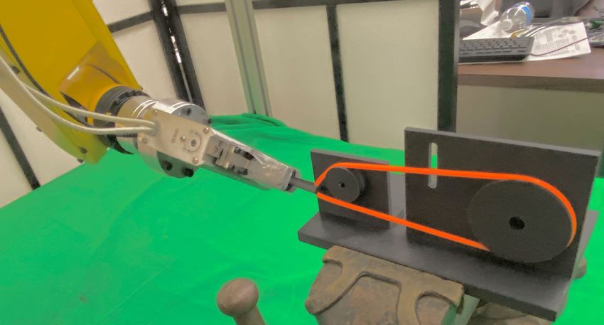
2) Results: Figure 7 provides the snapshots of the main
phases during the execution of a successful experiment. Fig-
ure 8 shows the trajectory of the gripper tip that corresponds
to K1 and the measured forces at the robot’s wrist along the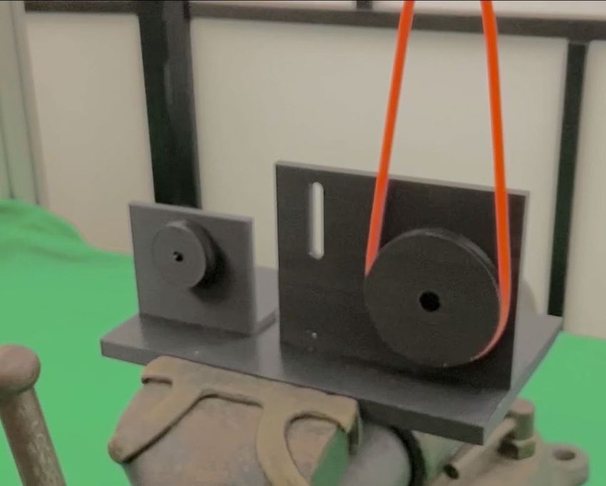
R EFERENCES                                        [23] M. Moll and L. E. Kavraki, “Path planning for deformable linear
                                                                                     objects,” IEEE Transactions on Robotics, vol. 22, no. 4, pp. 625–636,
 [1] Y. LeCun, Y. Bengio, and G. Hinton, “Deep learning,” nature, vol.               2006.
     521, no. 7553, pp. 436–444, 2015.                                          [24] D. Navarro-Alarcón, Y. Liu, J. G. Romero, and P. Li, “Model-
 [2] A. Krizhevsky, I. Sutskever, and G. E. Hinton, “Imagenet classification         free visually servoed deformation control of elastic objects by robot
     with deep convolutional neural networks,” Communications of the                 manipulators,” IEEE Transactions on Robotics, vol. 29, no. 6, pp.
     ACM, vol. 60, no. 6, pp. 84–90, 2017.                                           1457–1468, 2013.
 [3] D. Silver, J. Schrittwieser, K. Simonyan, I. Antonoglou, A. Huang,         [25] J. Zhu, B. Navarro, P. Fraisse, A. Crosnier, and A. Cherubini, “Dual-
     A. Guez, T. Hubert, L. Baker, M. Lai, A. Bolton et al., “Mastering              arm robotic manipulation of flexible cables,” in 2018 IEEE/RSJ
     the game of go without human knowledge,” nature, vol. 550, no. 7676,            International Conference on Intelligent Robots and Systems (IROS),
     pp. 354–359, 2017.                                                              2018, pp. 479–484.
 [4] S. Jin, X. Zhu, C. Wang, and M. Tomizuka, “Contact pose identifi-          [26] S. Jin, C. Wang, and M. Tomizuka, “Robust deformation model
     cation for peg-in-hole assembly under uncertainties,” arXiv preprint            approximation for robotic cable manipulation,” in 2019 IEEE/RSJ
     arXiv:2101.12467, 2021.                                                         International Conference on Intelligent Robots and Systems (IROS),
 [5] M. T. Mason, “Toward robotic manipulation,” Annual Review of                    2019, pp. 6586–6593.
     Control, Robotics, and Autonomous Systems, vol. 1, pp. 1–28, 2018.         [27] A. Nair, D. Chen, P. Agrawal, P. Isola, P. Abbeel, J. Malik, and
 [6] F. von Drigalski, C. Schlette, M. Rudorfer, N. Correll, J. Triyonoputro,        S. Levine, “Combining self-supervised learning and imitation for
     W. Wan, T. Tsuji, and T. Watanabe, “Robots assembling machines:                 vision-based rope manipulation,” 03 2017.
     Learning from the world robot summit 2018 assembly challenge,”             [28] N. Ratliff, M. Zucker, J. A. Bagnell, and S. Srinivasa, “Chomp:
     2019.                                                                           Gradient optimization techniques for efficient motion planning,” in
 [7] Y. F. Zheng, R. Pei, and C. Chen, “Strategies for automatic assembly            2009 IEEE International Conference on Robotics and Automation,
     of deformable objects,” in Proceedings. 1991 IEEE International                 2009, pp. 489–494.
     Conference on Robotics and Automation, 1991, pp. 2598–2603 vol.3.          [29] M. Kalakrishnan, S. Chitta, E. Theodorou, P. Pastor, and S. Schaal,
 [8] I. G. Ramirez-Alpizar, K. Harada, and E. Yoshida, “Motion planning              “Stomp: Stochastic trajectory optimization for motion planning,” in
     for dual-arm assembly of ring-shaped elastic objects,” in 2014 IEEE-            2011 IEEE International Conference on Robotics and Automation,
     RAS International Conference on Humanoid Robots, 2014, pp. 594–                 2011, pp. 4569–4574.
     600.                                                                       [30] J. Schulman, Y. Duan, J. Ho, A. Lee, I. Awwal, H. Bradlow, J. Pan,
 [9] J. Zhu, B. Navarro, R. Passama, P. Fraisse, A. Crosnier, and A. Cheru-          S. Patil, K. Goldberg, and P. Abbeel, “Motion planning with sequential
     bini, “Robotic manipulation planning for shaping deformable linear              convex optimization and convex collision checking,” The International
     objects with environmental contacts,” IEEE Robotics and Automation              Journal of Robotics Research, vol. 33, no. 9, pp. 1251–1270, 2014.
     Letters, vol. 5, no. 1, pp. 16–23, 2020.                                   [31] P. Foehn, D. Falanga, N. Kuppuswamy, R. Tedrake, and D. Scara-
[10] K. Tatemura and H. Dobashi, “Strategy for roller chain assembly with            muzza, “Fast trajectory optimization for agile quadrotor maneuvers
     parallel jaw gripper,” IEEE Robotics and Automation Letters, vol. 5,            with a cable-suspended payload.” RSS, 2017.
     no. 2, pp. 2435–2442, 2020.                                                [32] L. Manuelli, W. Gao, P. R. Florence, and R. Tedrake, “kpam: Keypoint
[11] T. Tang, C. Wang, and M. Tomizuka, “A framework for manipulating                affordances for category-level robotic manipulation,” 2019.
     deformable linear objects by coherent point drift,” IEEE Robotics and      [33] A. U. Raghunathan and L. T. Biegler, “An interior point method for
     Automation Letters, vol. 3, no. 4, pp. 3426–3433, 2018.                         mathematical programs with complementarity constraints (mpccs),”
[12] S. Jin, C. Wang, X. Zhu, T. Tang, and M. Tomizuka, “Real-time                   SIAM Journal on Optimization, vol. 15, no. 3, pp. 720–750, 2005.
     state estimation of deformable objects with dynamical simulation,”         [34] E. Todorov, T. Erez, and Y. Tassa, “Mujoco: A physics engine for
     in Workshop on Robotic Manipulation of Deformable Objects 2020                  model-based control,” in 2012 IEEE/RSJ International Conference on
     IEEE/RSJ International Conference on Intelligent Robots and Systems             Intelligent Robots and Systems, 2012, pp. 5026–5033.
     (IROS), 2020.                                                              [35] A. Wächter and L. T. Biegler, “On the implementation of an interior-
[13] M. Posa, C. Cantu, and R. Tedrake, “A direct method for trajectory op-          point filter line-search algorithm for large-scale nonlinear program-
     timization of rigid bodies through contact,” The International Journal          ming,” Math. Program., vol. 106, no. 1, p. 25–57, Mar. 2006.
     of Robotics Research, vol. 33, no. 1, pp. 69–81, 2014.
[14] P. Kolaric, D. Jha, A. Raghunathan, F. Lewis, M. Benosman,
     D. Romeres, and D. Nikovski, “Local policy optimization for
     trajectory-centric reinforcement learning,” in IEEE International Con-
     ference on Robotics and Automation (ICRA). IEEE, 2020, pp. 5094–
     5100.
[15] K. Yunt and C. Glocker, “Trajectory optimization of mechanical hybrid
     systems using sumt,” in 9th IEEE International Workshop on Advanced
     Motion Control, 2006. IEEE, 2006, pp. 665–671.
[16] R. Goebel, R. G. Sanfelice, and A. R. Teel, “Hybrid dynamical
     systems,” IEEE Control Systems Magazine, vol. 29, no. 2, pp. 28–
     93, 2009.
[17] R. Fierro, A. K. Das, V. Kumar, and J. P. Ostrowski, “Hybrid control of
     formations of robots,” in Proceedings 2001 ICRA. IEEE International
     Conference on Robotics and Automation (Cat. No.01CH37164), vol. 1,
     2001, pp. 157–162 vol.1.
[18] L. P. Kaelbling and T. Lozano-Pérez, “Hierarchical task and motion
     planning in the now,” in 2011 IEEE International Conference on
     Robotics and Automation, 2011, pp. 1470–1477.
[19] K. Yunt and C. Glocker, “A combined continuation and penalty method
     for the determination of optimal hybrid mechanical trajectories,” in
     IUTAM Symposium on Dynamics and Control of Nonlinear Systems
     with Uncertainty. Springer, 2007, pp. 187–196.
[20] K. Yunt, “An augmented lagrangian based shooting method for the
     optimal trajectory generation of switching lagrangian systems,” Dy-
     namics of Continuous, Discrete and Impulsive Systems Series B:
     Applications and Algorithms, vol. 18, no. 5, pp. 615–645, 2011.
[21] Z.-Q. Luo, J.-S. Pang, and D. Ralph, Mathematical programs with
     equilibrium constraints. Cambridge University Press, 2008.
[22] F. Lamiraux and L. E. Kavraki, “Planning paths for elastic objects
     under manipulation constraints,” The International Journal of Robotics
     Research, vol. 20, no. 3, pp. 188–208, 2001.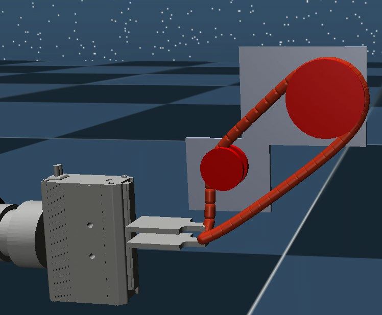
You can also read