Ultra-Reliable and Low-Latency Wireless Communication: Tail, Risk and Scale - arXiv
←
→
Page content transcription
If your browser does not render page correctly, please read the page content below
1

                                                     Ultra-Reliable and Low-Latency Wireless
                                                         Communication: Tail, Risk and Scale
                                           Mehdi Bennis, Senior Member IEEE, Mérouane Debbah, Fellow IEEE, and H. Vincent Poor,
                                                                                              Fellow IEEE
arXiv:1801.01270v2 [cs.IT] 23 Aug 2018

                                                                                                  Abstract

                                                     Ensuring ultra-reliable and low-latency communication (URLLC) for 5G wireless networks and beyond
                                              is of capital importance and is currently receiving tremendous attention in academia and industry. At
                                              its core, URLLC mandates a departure from expected utility-based network design approaches, in which
                                              relying on average quantities (e.g., average throughput, average delay and average response time) is no
                                              longer an option but a necessity. Instead, a principled and scalable framework which takes into account
                                              delay, reliability, packet size, network architecture, and topology (across access, edge, and core) and decision-
                                              making under uncertainty is sorely lacking. The overarching goal of this article is a first step to fill this void.
                                              Towards this vision, after providing definitions of latency and reliability, we closely examine various enablers
                                              of URLLC and their inherent tradeoffs. Subsequently, we focus our attention on a plethora of techniques
                                              and methodologies pertaining to the requirements of ultra-reliable and low-latency communication, as well
                                              as their applications through selected use cases. These results provide crisp insights for the design of low-
                                              latency and high-reliable wireless networks.

                                                                                               Index Terms

                                                     Ultra-reliable low-latency communication, 5G and beyond, resource optimization, mobile edge comput-
                                              ing.

                                                                                            I. Introduction

                                           The phenomenal growth of data traffic spurred by the internet-of-things (IoT) applications ranging from
                                         machine-type communications (MTC) to mission-critical communications (autonomous driving, drones and
                                         augmented/virtual reality) are posing unprecedented challenges in terms of capacity, latency, reliability, and
                                         scalability [1] [2],[3], [4]. This is further exacerbated by: i) a growing network size and increasing interactions
                                         between nodes; ii) a high level of uncertainty due to random changes in the topology; and iii) a heterogeneity
                                         across applications, networks and devices. The stringent requirements of these new applications warrant
                                         a paradigm shift from reactive and centralized networks towards massive, low-latency, ultra-reliable and

                                           M. Bennis is with the Centre for wireless communications, University of Oulu, 4500 Oulu, Finland, (e-mail:
                                         mehdi.bennis@oulu.fi). M. Debbah is with the Mathematical and Algorithmic Sciences Lab, Huawei France R&D, Paris, France,
                                         (e-mail: merouane.debbah@huawei.com). H. V. Poor is with the Department of Electrical Engineering, Princeton University,
                                         Princeton, NJ 08544 USA (e-mail: poor@princeton.edu).

                                         August 24, 2018                                                                                                      DRAFT
2

proactive 5G networks. Up until now, human-centric communication networks have been engineered with a
focus on improving network capacity with little attention to latency or reliability, while assuming few users.
  Achieving ultra-reliable and low-latency communication (URLLC) represents one of the major challenges
facing 5G networks. URLLC introduces a plethora of challenges in terms of system design. While enhanced
mobile broadband (eMBB) aims at high spectral efficiency, it can also rely on hybrid automatic repeat
request (HARQ) retransmissions to achieve high reliability. This is, however, not the case for URLLC due to
the hard latency constraints. Moreover, while ensuring URLLC at a link level in controlled environments is
relatively easy, doing it at a network level and over a wide area and in remote scenarios (e.g., remote surgery
[5], [6]) is notoriously difficult. This is due to the fact that for local area use cases latency is mainly due to
the wireless media access, whereas wide area scenarios suffer from latency due to intermediate nodes/paths,
fronthaul/backhaul and the core/cloud. Moreover, the typical block error rate (BLER) of 4G systems is
10−2 which can be achieved by channel coding (e.g., Turbo code) and re-transmission mechanisms (e.g., via
HARQ). By contrast, the performance requirements of URLLC are more stringent with a target BLER
of [10−9 − 10−5 ] depending on the use case [7]. From a physical-layer perspective, the URLLC design
is challenging as it ought to satisfy two conflicting requirements: low latency and ultra-high reliability
[8]. On the one hand, minimizing latency mandates the use of short packets which in turns causes a
severe degradation in channel coding gain [9], [10]. On the other hand, ensuring reliability requires more
resources (e.g., parity, redundancy, and re-transmissions) albeit increasing latency (notably for time-domain
redundancy). Furthermore, URLLC warrants a system design tailored to the unique requirements of different
verticals for which the outage capacity is of interest (as opposed to the Ergodic capacity considered in 4G
[11]). This ranges from users (including cell edge users) connected to the radio access network which must
receive equal grade of service [11], to vehicles reliably transmitting their safety messages [12] and industrial
plants whereby sensors, actuators and controllers communicate within very short cycles [13].
  If successful, URLLC will unleash a plethora of novel applications and digitize a multitude of verticals.
For instance, the targeted 1 ms latency time (and even lower) is crucial in the use of haptic feedback and
real-time sensors to allow doctors to examine patients’ bodies from a remote operating room [6]. Similarly,
the construction industry can operate heavy machinery remotely and minimize other potential hazards [14].
For sports fans, instead of watching NBA games on television, using a virtual reality (VR) headset allows to
have a 360-degree courtside view, feeling the intensity of the crowd from the comfort of the home [1]. The
end-to-end latency for XR (augmented, virtual and immersive reality) represents a serious challenge that
ought to be tackled. Likewise, ultra-high reliability in terms of successful packet rate delivery, which may
be as high as 1 − 10−5 (or even 1 − 10−9 ), will help automate factories, spearhead remote monitoring and
control [4]. Undoubtedly, these technological advances will only be possible with a scalable, ultra-reliable
and low-latency network.
In essence, as shown in Figure 1, URLLC can be broken down into three major building blocks, namely: (i)
risk, (ii) tail, and (iii) scale.
  •   Risk: risk is naturally encountered when dealing with decision making under uncertainty, when channels

August 24, 2018                                                                                            DRAFT
3

Figure 1. Anatomy of the URLLC building blocks, composed of tail, scale and risk alongside their unique characteristics. In
addition, mathematical tools tailored to the requirements of every block are highlighted therein.

      are time-varying and in the presence of network dynamics. Here, decentralized or semi-centralized
      algorithms providing performance guarantees and robustness are at stake, and notably game theory and
      reinforcement learning. Furthermore, Renyi entropy is an information-theoretic criterion that precisely
      quantifies uncertainty embedded in a distribution, accounting for all moments, encompassing Shannon
      entropy as a special case [15].
  •   Tail: the notion of tail behavior in wireless systems is inherently related to the tail of random traffic
      demand, tail of latency distribution, intra/inter-cell interference, and users that are at the cell edge,
      power-limited or in deep fade. Therefore, a principled framework and mathematical tools that charac-
      terize these tails focusing on percentiles and extreme events are needed. In this regard, extreme value
      theory [16], mathematical finance and network calculus are important methodologies.
  •   Scale: this is motivated by the sheer amount of devices, antennas, sensors and other nodes which pose
      serious challenges in terms of resource allocation and network design. Scale is highly relevant for mission-
      critical machine type communication use cases (e.g., industrial process automation) which are based on
      a large number of sensors, actuators and controllers requiring communication with very high reliability

August 24, 2018                                                                                                    DRAFT
4
and low end-to-end latency [4], [17]1 . In contrast to cumbersome and time-consuming Monte-Carlo
simulations, mathematical tools focused on large system analysis which provide a tractable formulation
and insights are needed. For this purpose, mean field (and mean field game) theory [18], statistical
physics and random matrix theory [19] are important tools.
The article is structured as follows: to guide the readers and set the stage for the technical part, definitions
of latency and reliability are presented in Section II. Section III provides a state-of-the-art summary of the
most recent and relevant works. Section IV delves into the details of some of the key enablers of URLLC,
and section V examines several tradeoffs cognizant of the URLLC characteristics. Next, Section VI presents
an overview of various tools and techniques tailored to the unique features of URLLC (risk, scale and tail).
Finally, we illustrate through selected use cases the usefulness of some of the methodologies in Section VII
followed by concluding remarks.
II. Definitions
A. Latency
• End-to-end (E2E) latency [20]: E2E latency includes the over-the-air transmission delay, queuing
delay, processing/computing delay and retransmissions, when needed. Ensuring a round-trip latency
of 1 ms and owing to the speed of light constraints (300 km/ms), the maximum distance at which a
receiver can be located is approximately 150 km.
• User plane latency (3GPP) [21]: defined as the one-way time it takes to successfully deliver an
application layer packet/message from the radio protocol layer ingress point to the radio protocol ingress
point of the radio interface, in either uplink or downlink in the network for a given service in unloaded
conditions (assuming the user equipment (UE) is in active state). The minimum requirements for user
plane latency are 4 ms for eMBB and 1 ms for URLLC assuming a single user.
• Control plane latency (3GPP) [21]: defined as the transition time from a most “battery efficient”
state (e.g., idle state) to the start of continuous data transfer (e.g. active state). The minimum require-
ment for control plane latency is 20 ms.
B. Reliability
In general, reliability is defined as the probability that a data of size D is successfully transferred within
a time period T . That is, reliability stipulates that packets are successfully delivered and the latency bound
is satisfied. However, other definitions can be encountered:
• Reliability (3GPP) [21]: capability of transmitting a given amount of traffic within a predetermined
time duration with high success probability. The minimum requirement for reliability is 1 − 10−5 success
probability of transmitting a layer 2 protocol data unit of 32 bytes within 1 ms.
1 Table 1 shows the scaling, reliability, latency and range for a wireless factory use case [17].
August 24, 2018 DRAFT5
• Reliability per node: defined as the transmission error probability, queuing delay violation probability
and proactive packet dropping probability.
• Control channel reliability: defined as the probability of successfully decoding the scheduling grant
or other metadata [22].
• Availability: defined as the probability that a given service is available (i.e., coverage). For instance,
99.99% availability means that one user among 10000 does not receive proper coverage [23].
We underscore the fact that URLLC service requirements are end-to-end, whereas the 3GPP and ITU
requirements focus on the one-way radio latency over the 5G radio network [21].
III. State-of-the-art and gist of recent work
Ensuring low-latency and ultra-reliable communication for future wireless networks is of capital impor-
tance. To date, no work has been done on combining latency and reliability into a theoretical framework,
although the groundwork has been laid by Polyanskiy’s development of bounds on block error rates for
finite blocklength codes [24], [25]. These works are essentially information-theoretic and overlook queuing
effects and other networking issues. Besides that, no wireless communication systems have been proposed
with latency constraints on the order of milliseconds with hundreds to thousands of nodes and with system
reliability requirements of 1 − 10−6 to 1 − 10−9 .
A. Latency
At the physical layer level, low-latency communication has been studied in terms of throughput-delay
tradeoffs [26]. Other theoretical investigations include delay-limited link capacity [27] and the use of network
effective capacity [28]. While interesting these works focus on minimizing the average latency instead of
the worst-case latency. At the network level, the literature on queue-based resource allocation is rich in
which tools from Lyapunov optimization, based on myopic queue-length based optimization are state-of-
the-art [29]. However, while stability is an important aspect of queuing networks, fine-grained metrics like
the delay distribution and probabilistic bounds (i.e., tails) cannot be addressed. Indeed a long-standing
challenge is to understand the non-asymptotic trade-offs between delay, throughput and reliability in wireless
networks including both coding and queuing delays. Towards this vision, the recent works of Al-Zubaidy et
al. [30] constitute a very good starting point, leveraging the framework of stochastic network calculus. Other
interesting works geared towards latency reduction at the network level include caching at the network edge
(base stations and user equipment) [31], [32], [33], [34], [32], [35], [36], the use of shorter transmission time
interval (TTI) [11], grant-free based non orthogonal multiple access [37], [8] and mobile edge computing [38],
[39], to mention a few.
B. Reliability
Reliable communication has been a fundamental problem in information theory since Shannon’s seminal
paper showing that it is possible to communicate with vanishing probability of error at non-zero rates [40].
August 24, 2018 DRAFT6
Several decades after saw the advent of many error control coding schemes for point-to-point communication
(Turbo, LDPC and Polar codes) [9]. In wireless fading channels, diversity schemes were developed to deal with
the deep fades stemming from multipath effects. For coding delays, error exponents (reliability functions)
characterize the exponential rates at which error probabilities decay as coding block-lengths become large
[41]. However, this approach does not capture sub-exponential terms needed to characterize the low delay
performance (i.e. the tails). Recent works on finite-block length analysis and channel dispersion [24], [25], [9]
help in this regard but do not address multiuser wireless networks nor interference-limited settings. At the
network level, reliability has been studied to complement the techniques used at the physical layer, including
automatic repeat request (ARQ) and its hybrid version (HARQ) at the medium access level. In these works,
reliability is usually increased at the cost of latency due to the use of longer blocklengths or through the use
of retransmissions.
Recently, packet duplication was shown to achieve high reliability in [2], [9], high availability using multi-
connectivity was studied in [23] in an interference-free scenario and stochastic network calculus was applied
in a single user and multiple input single output (MISO) setting in [42]. In terms of 5G verticals, challenges
of ultra-reliable vehicular communication were looked at in [12], [43], whereas mobile edge computing with
URLLC guarantees was studied in [44]. Network slicing for enabling ultra-reliable industrial automation was
examined in [4], and a maximum average rate was derived in [45] guaranteeing a signal-to-interference ratio.
Finally, a recent (high-level) URLLC survey article can be found in [46] highlighting the building principles
of URLLC.
Summary. Most of the current state-of-the-art has made a significant contribution towards understanding
the ergodic capacity and the average queuing performance of wireless networks focusing on large blocklength.
However, these works fall short of providing insights for reliability and latency issues and understanding their
non-asymptotic tradeoffs. In addition, current radio access networks are designed with the aim of maximizing
throughput while considering a few active users. Progress has been made in URLLC in terms of short-packet
transmission [9], [24] and other concepts such as shorter transmission time interval, network slicing, caching,
multi-connectivity, and so forth. However, a principled framework laying down the fundamentals of URLLC
at the network level, that is scalable and features a system design centered on tails is lacking.
IV. Key Enablers for URLLC
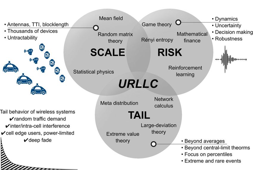
In this section, key enablers for low-latency and high-reliability communication are examined. An overview
of some of these enablers is highlighted in Figure 2, while Table I provides a comparison between 4G and
5G.
A. Low-Latency
A latency breakdown yields deterministic and random components that are either fixed or scale with the
number of nodes. While the deterministic component defines the minimum latency, the random components
impact the latency distribution and more specifically its tails. Deterministic latency components consist of
August 24, 2018 DRAFT7
the time to transmit information and overhead (i.e. parity bits, reference signals and control data), and
waiting times between transmissions. The random components include the time to retransmit information
and overhead when necessary, queuing delays, random backoff times, and other processing/computing delays.
In what follows, various enablers for low-latency communication are examined:
• Short transmission time interval (TTI), short frame structure and hybrid automatic repeat
request(HARQ): reducing the TTI duration (e.g., from 1 ms in LTE to 0.125 ms as in 5G new radio)
using fewer OFDM2 symbols per TTI and shortening OFDM symbols via wider subcarrier spacing as
well as lowering HARQ roundtrip time (RTT) reduce latency. This is because less time is needed to have
enough HARQ retransmissions to meet a reliability target and tolerate more queuing delay before the
deadline (owing to the HARQ retransmissions constraints). Furthermore, reducing the OFDM symbol
duration increases subcarrier spacing and hence fewer resource blocks are available in the frequency
domain causing more queuing effect. On the flipside, shorter TTI duration introduces more control
overhead thereby reducing capacity (lower availability of resources for other URLLC data transmissions).
This shortcoming can be alleviated using grant-free transmission in the uplink. In the downlink, longer
TTIs are needed at high offered loads to cope with non-negligible queuing delays [11].
• eMBB/URLLC multiplexing: Although a static/semi-static resource partitioning between eMBB
and URLLC transmissions may be preferable in terms of latency/reliability viewpoint, it is inefficient
in terms of system resource utilization, calling for a dynamic multiplexing solution [11]. Achieving
high system reliability for URLLC requires more frequency-domain resources to be allocated to an
uplink (UL) transmission instead of boosting power on narrowband resources. This means wideband
resources are needed for URLLC UL transmission to achieve high reliability with low latency. In addition,
intelligent scheduling techniques to preempt other scheduled traffic are needed when a low-latency packet
arrives in the middle of the frame (i.e., puncturing the current eMBB transmission). At the same time,
the eMBB traffic should be minimally impacted when maximizing the URLLC outage capacity. A recent
work towards this direction can be found in [47] as well as a recent application in the context of virtual
reality [48].
• Edge caching, computing and slicing: pushing caching and computing resources to the network edge
has been shown to significantly reduce latency [49], [50]. This trend will continue unabated with the
advent of resource-intensive applications (e.g., augmented and virtual reality) and other mission-critical
applications (e.g., autonomous driving). In parallel to that, network slicing will also play a pivotal role
in allocating dedicated caching, bandwidth and computing resources (slices).
• On-device machine learning and artificial intelligence (AI) at the network edge: Machine
learning (ML) lies at the foundation of proactive and low-latency networks. Traditional ML is based
on the precept of a single node (in a centralized location) with access to the global dataset and a
massive amount of storage and computing, sifting through this data for classification and inference.
22 OFDM symbols = 71.43 microseconds with a spacing of 30 KHz.
August 24, 2018 DRAFT8
Nevertheless, this approach is clearly inadequate for latency-sensitive and high-reliability applications,
sparking a huge interest in distributed ML (e.g, deep learning coined by Lecun et. al. [51]). This mandates
a novel scalable and distributed machine learning framework, in which the training data describing the
problem is stored in a distributed fashion across a number of interconnected nodes and the optimization
problem is solved collectively. This constitutes the next frontier for ML, also referred to as AI-on-edge
or on-device ML [52]. Our preliminary work in this direction can be found in [53].
• Grant-free versus grant-based access: This relates to dynamic uplink scheduling or contention-
based access for sporadic/bursty traffic versus persistent scheduling for periodic traffic. Fast uplink
access is advocated for devices on a priori basis at the expense of lower capacity (due to resource pre-
allocation). For semi-persistent scheduling unused resources can be reallocated to the eMBB traffic. In
another solution referred to as group-based semi-persistent scheduling, contention based access is carried
out within a group of users with similar characteristics, thereby minimizing collisions within the group
[54]. In this case the base station controls the load and dynamically adjusts the size of the resource pool.
For retransmissions, the BS could also proactively schedule a retransmission opportunity shared by a
group of UEs with similar traffic for better resource utilization. On the other hand, grant-free access
shortens the procedure for uplink resource assignment, whereby the reservation phase is skipped.
• Non-orthogonal multiple access (NOMA): NOMA (and its variants) reduces latency by supporting
far more users than conventional orthogonal-based approaches leveraging power or code domain multi-
plexing in the uplink then using successive interference cancellation (SIC), or more advanced receiver
schemes (e.g., message passing or Turbo reception). However, issues related to imperfect channel state
information (CSI), user ordering, processing delay due to multiplexing and other dynamics which impact
latency (and reliability) are not well understood.
• Low/Medium-earth orbit (LEO/MEO) satellites and unmanned aerial vehicles (UAVs):
Generally, connecting terrestrial base stations to the core network necessitates wired backhauling3.
However, wired connections are expensive and sometimes infeasible due to geographical constraints such
as remote areas. In this case, UAVs can enable a reliable and low-latency wireless backhaul connectivity
for ground networks [3], [57], [58]. Furthermore, for long-range applications or in rural areas, LEO
satellites are the only way to reduce backhaul latency in which a hybrid architecture composed of
balloons, LEOs/MEOs and other stratospheric vehicles are low-latency communication enablers [59].
• Joint flexible resource allocation for uplink/downlink: for time division duplex (TDD) systems, a
joint uplink/downlink allocation and the interplay of time slot length versus the switching cost (or turn
around) is needed. This topic has been studied in the context of LTE-A. Here, for frequency division
duplex (FDD) both LTE evolution and the new radio (NR) are investigated, whereas for TDD only NR
is investigated since LTE TDD is not considered for URLLC enhancements.
3 In addition, backhaul provisioning can be done by leveraging massive MIMO, whereby instead of deploying more base stations,
some antenna elements can be used for wireless backhauling [55], [56].
August 24, 2018 DRAFT9
Reliability (1 − 10−x )
-2
ENABLERS Best Effort
• Short TTI
• Caching Low-Latency
• Densification Communication
• Grant-free (LLC) ITS
• UAV/UAS
-5
• Non orthogonal multiple
access (NOMA)
• MEC/FOG/MIST Factory 2.0
• Network coding
• Machine learning -9 Ultra-Reliable Communication
URLLC (URC)
• Slicing Latency (ms)
0.1 1 10 100
ENABLERS ENABLERS
• Short TTI • Finite blocklength
• Spatial diversity • Packet duplication
• Network coding • HARQ
• Caching, MEC • Multi-connectivity
• Multi-connectivity • Network coding
• Grant-free + NOMA • Spatial diversity
• Machine learning • Slicing
• Slicing
Figure 2. A breakdown of the key enablers for low latency and high reliability.
B. Reliability
The main factors affecting reliability stem from: i) collisions with other users due to uncoordinated
channel access; ii) coexistence with other systems in the same frequency bands; iii) interference from users in
adjacent channels; iv) Doppler shifts from moving devices, v) difficulty of synchronization, outdated channel
state information, time-varying channel effects or delayed packet reception. Reliability at the physical layer
level (typically expressed in block error rate) depends on factors such as the channel, constellation, error
detection codes, modulation technique, diversity, retransmission mechanisms, etc. A variety of techniques
to increase reliability include using low-rate codes to have enough redundancy in poor channel conditions,
retransmissions for error correction, and ARQ at the transport layer. Crucially, diversity and beamforming
provide multiple independent paths from the transmitter to the receiver and to boost the received signal-
to-noise ratio (SNR). Frequency diversity occurs when information is transmitted over a frequency-selective
channel whereas time diversity occurs when a forward error correction (FEC) codeword is spread out over
August 24, 2018 DRAFT10
many coherence times so that it sees many different channels (for e.g., using HARQ). Multi-user diversity
arises when a transmission is relayed by different users from the source to the destination. In what follows,
various enablers for reliability are discussed.
• Multi-connectivity and harnessing time/frequency/RATs diversity: while diversity is a must,
time diversity is not a viable solution when the tolerable latency is shorter than the channel coherence
time or when the reliability requirements are very stringent. On the other hand frequency diversity
may not scale with the number of users/devices, making spatial diversity the only solution. In this
regard, multi-connectivity is paramount in ensuring high-reliable communication. Nevertheless several
fundamental questions arise, such as what is the optimal number of links needed to ensure a given
reliability target? issues of correlated links versus independent links; how to deal with synchronization,
non-reciprocity issues, and other imperfections?
• Multicast: when receivers are interested in the same information (e.g., mission-critical traffic safety
or a common field-of-view in virtual reality), multicast is more reliable than using unicast. However
reliability can be sensitive to the coverage range, what modulation and coding scheme (MCS) is used
within the multicast group and who determines the MCS? Moreover, the usefulness of multicast will
depend on whether transmission is long-range or short-range as the performance is inherently limited
by cell edge users.
• Data replication (contents and computations): needed when coordination among nodes is not
possible, when a low-rate backhaul is needed for coordination or due to lack of channel state information.
This comes at the expense of lower capacity. One solution could be to replicate the same data until
receiving an acknowledgement in the case of HARQ.
• HARQ + short frame structure, short TTI: improve outage capacity via sufficient retransmissions
to achieve high reliability. Here an optimal MCS level selection with the constraint of required reliability
and latency (not necessarily optimized for spectral efficiency) is an open research problem.
• Control channel design: Unlike LTE where the focus was primarily on protecting data but not the
control channel, ensuring high reliability for the control channel is a must. This can be done by sending
the delay budget information from the user to the base station (BS) in the control channel, such that on
the downlink the BS can select the optimal modulation coding scheme based on both channel quality
indicator (CQI)4 report and remaining latency budget. In addition, replicating the same data until
receiving an acknowledgement for HARQ can be envisaged at the cost of wasting resources.
• Manufacturing diversity via network coding and relaying: when time diversity cannot be relied
upon (due to extreme latency and reliability constraints) or in the presence of extreme fading events,
manufacturing diversity and robustness are key for ensuring URLLC. For instance, in industrial au-
tomation exploiting multi-user diversity and network coding using simultaneous relaying to enable a
4 Adaptive channel quality indicator (CQI) reporting is key in URLLC whereby more resources can be allocated to enhance
the reliability or changing the encoding rate of the CQI.
August 24, 2018 DRAFT11
Table I
4G vs. 5G (in a nutshell)
4G 5G
Metadata important crucial
Packet size Long (MBB) Short (URLLC)- Long (eMBB)
Design Throughput-centric, Average delay good enough Latency and reliability centric / tails MATTER
Reliability 95% or less 1 − 10−x x = [3, 4, 5, 6, 8, 9]
Rate Shannonian (long packets) Rate loss due to short packets
Delay violation Exponential decay using effective bandwidth Faster decay than exponential
Latency 15 ms RTT based on 1 ms subframe 1 ms and less, shorter TTI, HARQ RTT
Queue size unbounded bounded
Frequency bands sub-6GHz Above- and sub-6GHz (URLLC at sub-6GHz)
Scale A few users/devices billion devices
two-way reliable communication without relying on time and frequency diversity is important due to
the cycle time constraints, channel and network dynamics [4].
• Network slicing: it refers to the process of slicing a physical network into logical sub-networks opti-
mized for specific applications, in which the goal is to allocate dedicated resources for verticals of interest,
such as vehicle-to-vehicle communication and industrial automation [60]. Constructing network slices
with stringent reliability guarantees for these mission-critical applications is a daunting task due to
the difficulties in modeling and predicting queuing delays with very high accuracy. For instance, in
the industrial automation scenario, owing to its diverse set of application requirements, one slice could
be allocated for a high-definition video transmission between a person remotely monitoring a process
(or robot), and another slice to provide an ultra-reliable transmission between sensors, controllers and
actuators [4], [13].
• Proactive packet drop: when channel is in a deep fade, packets that cannot be transmitted even with
the maximal transmit power can be discarded proactively at the transmitter. Similarly, packet drop can
arise at the receiver when the maximum number of re-transmissions is reached. This is different than
the enhanced mobile broadband scenarios based on infinite queue buffers. In this case either spatial
diversity should be used or resources need to be increased.
• Space-time block codes: Orthogonal space-time block coding has been a very successful transmit
diversity technique because it achieves full diversity without CSI at the transmitter and need for joint
decoding of multiple symbols. Typically, it is characterized by the number of independent symbols Ns
transmitted over T time slots; the code rate is Rc = Ns /T . In the presence of channel imperfection,
orthogonal space-time block coding can outperform other diversity-seeking approaches such as the
maximum ratio transmission.
August 24, 2018 DRAFT12
V. Fundamental Trade-offs in URLLC
URLLC features several system design trade-offs which deserve a study on their own. In what follows, we
zoom in on some of these tradeoffs:
Finite versus large blocklength: In low-latency applications with small blocklength, there is always a
probability that transmissions fail due to noise, deep fading, collision, interference, and so forth. In this case,
the maximum coding rate Ri (n, ǫ) = k/n is lower than the Shannon rate, when transmitting k information
bits using coded packets spanning n channel uses. Furthermore, for high reliability, data must be encoded
at a rate which is significantly lower than the Shannon capacity5 . A number of works have shown that the
Shannon capacity model significantly overestimates the delay performance for such applications, which would
lead to insufficient resource allocations [42]. Despite a huge interest in the field [24], [9], a solid theoretical
framework for modeling the performance of such systems due to short time spans, finite blocklength and
interference is needed.
Spectral efficiency versus latency: achieving low latency incurs a spectral efficiency penalty (due to
HARQ and shorter TTI). A system characterization of spectral efficiency versus latency in a multiple access
and broadcast system taking into account: (a) bursty packet arrivals, (b) mixture of low latency and delay
tolerant traffic, and (c) channel fading and multipath is missing. Low latency transmission on the uplink
can be achieved with single shot slotted Aloha type transmission strategy where the device sends data
immediately without incurring the delay associated with making a request and receiving a scheduling grant.
Device energy consumption versus latency: A fundamental tradeoff that needs to be characterized is
the relationship between device energy consumption and latency. In wireless communications, devices need
to be in sleep or deep sleep mode when they are not transmitting or receiving to extend battery life. Since
applications from the network may send packets to the device, the device needs to wake up periodically to
check if packets are waiting. The frequency with which the device checks for incoming packets determines
latency of the packets as well as the energy consumption. The more frequent the lower the latency but higher
the energy consumption. Similarly, when reliability is deteriorated retransmissions are required, which means
more energy consumption is needed to guarantee a target reliability.
Energy expenditures versus reliability: higher reliability requires having several low-power transmissions
instead of one high-reliable and high-power transmission as shown in [14]. However, this depends on the
diversity order that can be achieved and whether independent or correlated fading is considered.
Reliability versus latency and rate: generally speaking, higher reliability requires higher latencies due
to retransmissions, but there could also be cases where both are optimized. In terms of data rates, it was
shown in [45] that guaranteeing higher rates incur lower reliability and vice-versa.
SNR versus diversity: fundamental questions include: how does the SNR requirement decrease as a
function of network nodes and diversity order? Does the use of higher frequency bands help provide more/less
5 If the blocklength is large, no errors occur and the achievable rate is equal to the well-known Shannon capacity, Ri =
log2 (1 + SNR) for AWGN channels.
August 24, 2018 DRAFT13
diversity? How much SNR is needed to compensate for time-varying channels, bad fading events, etc. Besides,
how does reliability scale with the number of links/nodes?
Short/long TTI versus control overhead: TTI duration should be adjusted according to user-specific
radio channel conditions and quality of service requirements to compensate for the control overhead. As
shown in [37], as the load increases the system must gradually increase the TTI size (and consequently
the spectral efficiency) to cope with non-negligible queuing delay, particularly for the tail of the latency
distribution. Hence using different TTI sizes to achieve low latency, depending on the offered load and the
percentile of interest is needed.
Open versus closed loop: For closed loop if more resources are used for channel training and estimation,
more accurate CSI is obtained albeit low data resources. For open loop a simple broadcast to all nodes
may be sufficient but requires more downlink resources. In this case building diversity by means of relay
nodes or distributed antennas is recommended. This problem needs to be revisited in light of short packet
transmissions.
User density versus dimensions (antennas, bandwidth and blocklength): Classical information
theory rooted in infinite coding blocklength assumes a fixed (and small) number of users, where fundamental
limits such as the coding blocklength n → ∞ are studied. In the large-scale multiuser scenario, n → ∞ is
taken before the number of users k → ∞. In massive machine type communication, a massive number of
devices with sporadic traffic need to share the spectrum in a given area which means k > n. In this case,
allowing n → ∞ while fixing k may be inaccurate and provides little insight. This warrants a rethinking of
the assumption of fixed population of full buffer users. A step towards this vision is many-user information
theory where the number of users increases without bound with the blocklength, as proposed in [61].
VI. Tools and Methodologies for URLLC
As alluded to earlier, URLLC mandates a departure from expected utility-based approaches relying on
average quantities. Instead, a holistic framework which takes into account end-to-end delay, reliability, packet
size, network architecture/topology, scalability and decision-making under uncertainty is needed. In addition,
fundamental system design and algorithm principles central to URLLC are at stake. Next, following-up on
the breakdown in Figure 1, we identify a (non-exhaustive) set of tools and methodologies which serve this
purpose.
A. RISK
1) Risk-sensitive learning and control: The notion of “risk” is defined as the chance of a huge loss
occurring with very low probability. In this case instead of maximizing the expected payoff (or utility), the
goal is to mitigate the risk of the huge loss. While reinforcement learning aims at maximizing the expected
utility of an agent (i.e., a transmitting node), risk-sensitive learning is based on the fact that the utility is
modified so as to incorporate the risk (e.g., variance, skewness, and other higher order statistics). This is done
August 24, 2018 DRAFT14
by exponentiating the agent’s cost function before taking the expectation, yielding higher order moments.
More concretely, the utility function of an agent i is given by:
1 h i
ri,µi = log Ex (eµi ui (xi ) ) , (1)
µi
where µi is the risk-sensitivity index and xi is the agent’s transmission strategy. By doing a Taylor approx-
imation around µi = 0 we get:
µi
ri,µi ≈ E[ui ] + var(ui ) + O(µi ). (2)
2
Moreover,
ri,µi − 1 1h i
lim = lim Exi (eµi ui (xi ) ) − 1 = Exi (ui ). (3)
µi →0 µi µi →0 µi
In risk-sensitive reinforcement learning, every agent needs to first estimate its own utility function r̂i,µi
over time based on a (possibly delayed or imperfect) feedback before updating its transmission probability
distribution xi . The utility estimation of agent i when choosing strategy xi is typically given by:
eµi ui,t+1 − 1
r̂i,t+1 (xi ) = r̂i,t (xi ) + λt − r̂i,t (xi ) , (4)
µi
where λt is a learning parameter. The application of risk-sensitive learning in the context of millimeter-wave
communication is given in Section VIII.A.
2) Mathematical finance and portfolio optimization: Financial engineering and electrical engineer-
ing are seemingly different areas that share strong underlying connections. Both areas rely on statistical
analysis and modeling of systems and the underlying time series. Inspired from the notion of risk in mathe-
matical finance, we examine various risk measures, such as the value-at-risk (VaR), conditional VaR (CVaR),
entropic VaR (EVaR) and mean-variance.
• Value-at-Risk (VaR): Initially proposed by J.-P. Morgan, VaR was developed in response to financial
disasters of the 1990s and played a vital role in market risk management. By definition VaR is the worst
loss over a target horizon with a given level of confidence such that for 0 < α ≤ 1:
n o
VaR1−α (X) = inf t : Prob(X ≤ t) ≥ 1 − α (5)
t
−1
which can also be expressed as: VaRα (X) = FX (1 − α).
• Conditional VaR: CVaR measures the expected loss in the right tail given a particular threshold has
been crossed. The CVaR is defined as the conditional mean value of a random variable exceeding a
particular percentile. This precisely measures the risky realizations, as opposed to the variance that
simply measures how spread the distribution is. Moreover CVaR overcomes the caveat of VaR due to
the lack of control of the losses incurred beyond the threshold. Formally speaking, it holds that:
n 1 o
CVaR1−α (X) = inf t + E[(X − t)+ ]
t α
1 α
Z
= VaR1−t (X)dt = E(X|X > VaR1−α ). (6)
α 0
August 24, 2018 DRAFT15
• Entropic VaR (EVaR): EVaR is the tightest upper bound one can find using the Chernoff inequality
for the VaR, where for all z ≥ 0:
Prob(X ≥ a) ≤ e−az MX (z) (7)
MX (z) = E(ezX ) is the moment generating function (MGF) of random variable X.
EVaR1−α (X) = inf z −1 log(MX (z))/α (8)
z>0
By solving the equation e−za MX (z) = α with respect to a for α ∈ [0, 1], we get
aX (α, z) = z −1 log(MX (z))/α. (9)
EVaR is an upper bound for the CVaR and its dual representation is related to the Kullback-Leibler
divergence [62]. Moreover, we have that:
log EP (eX ) = sup EQ (X) − DKL (Q||P ) (10)
Q VaR1−α ) = E(Y + d|X > d) = E(Y |X > d) + d, (11)
where Y |X>d = X − d. Letting α → 0 and as per Theorem 2, Y can be approximated by a generalized
Pareto distribution random variable whose mean is equal to CVaR1−α (X) − VaR1−α (X).
• Markowitz’s mean-variance (MV): MV is one of the most popular risk models in modern finance
(also referred to as Markowitz’s risk-return model), in which the value of an investment is modeled
as a tradeoff between expected payoff (mean return) and variability of the payoff (risk). In a learning
context, this entails learning the variance of the payoff from the feedback as follows. First, the variance
estimator of agent i at time t is given by:
t
1X
v̂i,t = (ri,t′ − r̂i,t′ )2 , (12)
t ′
t =1
after which the variance is estimated as:
v̂i,t+1 = v̂i,t + βt (ri,t′ − r̂i,t′ )2 − v̂i,t . (13)
and βt is a learning parameter. Once the variance is estimated, principles of reinforcement learning can be
readily applied [63].
Remark: Risk-sensitivity is also a common theme in prospect theory (PU), in which the notion of risk arises
through nonlinear distortions of the value function and probabilities. PU dates back to the Nobel prize work
of Kahnemann and Tversky [64], whose postulates depart from expected utility theory and risk-neutrality.
August 24, 2018 DRAFT16
Instead, it is based on two factors, namely the distortion of probabilities in the probability weighting function
and the shape in the value function. This is motivated by the fact that people put too much weight on small
probabilities and too little weight on large probabilities. Mathematically, this is captured by a value function
and probability weighting function whose shape is determined by a set of parameters. The application of
prospect theory in wireless communication can be found in cognitive radios [65] and smart grid [66].
B. TAIL
1) Extreme value theory (EVT): Latency and reliability are fundamentally about “taming the tails”
and going beyond “central-limit theorems”. In this regard, EVT provides a powerful and robust framework to
fully characterize the probability distributions of extreme events and extreme tails of distributions. EVT has
been developed during the twentieth century and is now a well-established tool to study extreme deviations
from the average of a measured phenomenon. EVT has found many applications in oceanography, hydrology,
pollution studies, meteorology, material strength, highway traffic and many others (for a comprehensive
survey on EVT, see [16]). EVT is built around the two following Theorems:
Theorem 1 (Fisher-Tippett-Gnedenko theorem for block maxima [16]). Given n independent sam-
ples, X1 , · · · , Xn , from the random variable X, define Mn = max{X1 , · · · , Xn }. As n → ∞, we can
approximate the cumulative distribution function (CDF) of Mn as
ξ(z−µ)
−1/ξ
− 1+
FMn (z) = Prob(Mn ≤ z) ≈ G(z; µ, σ, ξ) = e σ , (14)
where G(z; µ, σ, ξ), defined on {z: 1 + ξ(z − µ)/σ > 0}, is the generalized extreme value (GEV) distribution
characterized by the location parameter µ ∈ R, the scale parameter σ > 0, and the shape parameter ξ ∈ R.
Theorem 2 (Pickands-Balkema-de Haan theorem for exceedances over thresholds [16]). Consider
the distribution of X conditionally on exceeding some high threshold d. As the threshold d closely approaches
−1
FX (1), i.e., d → sup{x: FX (x) < 1}, the conditional CDF of the excess value Y = X − d > 0 is
−1/ξ
ξy
FY |X>d (y) = Prob(X − d ≤ y|X > d) ≈ H(y; σ̃, ξ) = 1 − 1 + , (15)
σ̃
where H(y; σ̃, ξ), defined on {y: 1 + ξy/σ̃ > 0}, is the generalized Pareto distribution (GPD). Moreover, the
characteristics of the GPD depend on the scale parameter σ̃ > 0 and the shape parameter ξ ∈ R. The location
and scale parameters in (14) and (15) are related as per σ̃ = σ + ξ(d − µ) while the shape parameters ξ in
both theorems are identical.
While Theorem 1 focuses on the maximal value of a sequence of variables, Theorem 2 aims at the values
of a sequence above a given threshold. Both theorems asymptotically characterize the statistics of extreme
events and provide a principled approach for the analysis of ultra-reliable communication, i.e., failures with
extreme low probabilities. A direct application of EVT to mobile edge computing scenarios is found in
Section VII.D. Other applications of EVT in vehicular communication can be found in [67], [53].
August 24, 2018 DRAFT17
2) Effective bandwidth: Effective bandwidth is a large-deviation type approximation defined as the
minimal constant service rate needed to serve a random arrival under a queuing delay requirement [28]. Let
a(t) and q(t) be the number of arrivals at time t and the number of users in the queue at time t, respectively.
Assume the queue size is infinite and the server can serve c(t) users per unit of time. c(t) is referred to as
server capacity at time t and the queue is governed by the following equation:
+
q(t + 1) = q(t) + a(t + 1) − c(t + 1) (16)
Moreover, let:
1
ΛA (θ) = lim log E[eθA(0,t) ] (17)
t→∞ t
for all θ ∈ R, and ΛA (θ) is differentiable. Let Λ∗A (α) be the Legendre transform of ΛA (θ), i.e.,
Λ∗A (α) = sup θα − ΛA (θ) .
(18)
θ
Likewise let Λ∗C (α) be the Legendre transform of ΛC (θ). We seek the decay rate of the tail distribution of
the stationary queue length. This is given in [28] which states that if there exists a unique θ∗ > 0 such that
Λ∗A (α) + Λ∗C (−α) = 0, (19)
then it holds that:
log Pr(q(∞ ≥ x))
lim = −θ∗ . (20)
x→∞ x
In particular, for fixed capacity c(t) = c for all t, we have that:
ΛA (θ∗ )
=c (21)
θ∗
ΛA (θ ∗ )
θ∗ is called the effective bandwidth of the arrival process subject to the condition that the tail distribution
of the queue length has the decay rate θ∗ .
Remark: since the distribution of queuing delay is obtained based on large deviation principles, the effective
bandwidth can be used for constant arrival rates, when the delay bound is large and the delay violation
probability is small. This raises the question on the usefulness and correctness of using the effective bandwidth
in solving problems dealing with finite packet/queue lengths and very low latencies.
3) Stochastic network calculus (SNC): SNC considers queuing systems and networks of systems with
stochastic arrival, departure, and service processes, where the bivariate functions A(τ, t), D(τ, t) and S(τ, t)
for any 0 ≤ τ ≤ t denote the cumulative arrivals, departures and service of the system, respectively, in
the interval [τ, t). The analysis of queuing systems is done through simple linear input-output relations.
In the bit domain it is based on a (min, +) dioid algebra where the standard addition is replaced by the
minimum (or infimum) and the standard multiplication replaced by addition. Similar to the convolution
and deconvolution in standard algebra, there are definitions for convolution and deconvolution operators in
the (min, +) algebra and the convolution and deconvolution operators in (min, +)-algebra are often used
for performance evaluation. Finally, observing that the bit and SNR domains are linked by the exponential
function, arrival and departure processes are transferred from the bit to the SNR domain. Then backlog
August 24, 2018 DRAFT18
and delay bounds are derived in the transfer domain using the (min, ×) algebra before going back to the bit
domain to obtain the desired performance bounds.
Define the cumulative arrival, service and departure processes as:
t−1
X t−1
X t−1
X
A(τ, t) = ai , S(τ, t) = si , D(τ, t) = di (22)
i=τ i=τ i=τ
The backlog at time t is given by B(t) = A(0, t) − D(0, t). Moreover, the delay W (t) at time t, i.e. the
number of slots it takes for an information bit arriving at time t to be received at the destination, is
n o
W (t) = inf u ≥ 0 : A(0, t)/D(0, t + u) ≤ 1 and the delay violation probability is given by
Λ(w, t) = Prob(W (t) > w) (23)
SNC allows to obtain bounds on the delay violation probability based on simple statistical characterizations
of the arrival and service processes in terms of their Mellin transforms. First by converting the cumulative
processes in the bit domain through the exponential function, the corresponding processes in the SNR domain
are: A(τ, t) = eA(τ,t) , S(τ, t) = eS(τ,t) , D(τ, t) = eD(τ,t) . From these definitions, an upper bound on the
delay violation probability can be computed by means of the Mellin transforms of A(τ, t) and S(τ, t):
pv (w) = inf {K(s, −w)} ≥ Λ(w) = Prob(W > w) (24)
s>0
where K(s, −w) is the so-called steady-state kernel, defined as
τ
X
K(s, −w) = lim MA (1 + s, t + w, t) · MS (1 − s, t + w, τ ) (25)
t→∞
u=0
and MX (s) = E[X s−1 ] denotes the Mellin6 transform of a nonnegative random variable X, for any s.
Analogous to [30] we consider (σ(s), ρ(s))-bounded arrivals where the log-MGF of the cumulative arrivals
in the bit domain is bounded by
1
log E[esA(τ,t) ] ≤ ρ(s).(t − τ ) + σ(s). (26)
s
This characterization can be viewed as a probabilistic extension of a traffic flow that is deterministically
regulated by a token bucket with rate ρ and burst size σ. To simplify the notation, we restrict the following
analysis to values (σ, ρ) that are independent of s, which is true for constant arrivals. Subsequently, the
Mellin transform of the SNR-domain arrival process can be upper-bounded by:
MA (s, τ, t) = E[A(τ, t)s−1 ] ≤ e(s−1)(ρ.(t−τ )+σ) (27)
6 By setting s = θ + 1, we obtain the effective bandwidth and MGF-based network calculus.
August 24, 2018 DRAFT19
Assuming the cumulative arrival process in SNR domain to have stationary and independent increments,
the steady-state kernel for a fading wireless channel is given by:
Mw
g(γ) (1 − s)
K(s, −w) = (7)
1 − Mα (1 + s)Mg(γ) (1 − s)
for any s > 0, under the stability condition Mα (1 + s)Mg(γ) (1 − s) < 1. The delay bound (24) thus reduces
to
Mw
g(γ) (1 − s)
pv (w) = inf (28)
s>0 1 − Mα (1 + s)Mg(γ) (1 − s)
4) Meta distribution: The meta distribution is a fine-grained key performance metric of wireless sys-
tems, first introduced in [68] which provides a mathematical foundation for questions of network densification
under strict reliability constraints. As such, the meta distribution is a much sharper and refined metric than
the standard success probability, which is easily obtained as the average over the meta distribution. By
definition, the meta distribution F̄Ps (x) is the complementary cumulative distribution function (CCDF) of
the random variable
Ps (θ) , P(SIR0 > θ | Φ) = Eh [1{SIR0 >θ} ] (29)
which is the CCDF of the conditional signal-to-interference ratio (SIR) of the typical user (′ 0′ ) given the
points processes Φ and conditioned on the desired transmitter to be active. The meta distribution is formally
given by [69]:
F̄Ps (x) , P0 (Ps (θ) > x), θ ∈ R+ , x ∈ [0, 1] . (30)
P0 is the Palm measure. Interestingly, the moments Mb reveal interesting properties of the meta distribution,
in which Z 1
M1 = F̄ (θ, x)dx and var(Ps (θ)) = M2 − M12 . (31)
0
is the standard success probability and variance, respectively.
Since all point processes in the model are ergodic, the meta distribution can be interpreted as the fraction
of the active links whose conditional success probabilities are greater than x. A simple approach to calculate
the meta distribution is to approximate it with the beta distribution, which requires only the first and second
moments. Recent applications of the Meta distribution can be found in [45] for industrial automation, [70]
in the context of V2V communication, and millimeter-wave device-to-device networks in [71].
C. SCALE
1) Statistical physics: Current wireless systems can support tens to hundreds of nodes with latency
constraints on the order of seconds and with moderate reliability. Nonetheless, these do not scale well to
systems with thousands to millions of nodes as envisaged in massive MTC or ultra-dense networks. Solving
resource allocation problems in large-scale network deployments is intractable and requires cumbersome
August 24, 2018 DRAFT20
Monte-Carlo simulations lacking fundamental insight. Here, cutting-edge methods from statistical physics
such as the replica method and cavity methods, provide fundamental insights and guidelines for the design
of massive and ultra-reliable networks.
Interactions between particles (e.g. atoms, gases or neurons) is a common theme in the statistical physics
literature [72], [73], [74]. Here, instead of analyzing the microscopic network state, one is concerned with the
macroscopic state requiring only a few parameters. By invoking this analogy and modeling network elements
as particles, a network cost function Φ(x, h) which captures the interactions between network elements is
referred to as the Hamiltonian H(x ∈ X ) over the state space X and h.
One of the underlying principles of statistical physics is to find the lowest energy of a system with the
aid of the partition sum Z = x∈X e−βH(x) , summing over all the states of the Boltzmann factors e−βH(x)
P
1
at a given fictitious temperature β → 0. By adopting the concept of quenched disorder7, the network can
be replicated to solve the interactions of infinitely large number of network elements, in which the ground
state over Eh [Φ⋆ (h)] is found via the replica method. Here, Φ⋆ (h) is the optimal network cost with the
exact knowledge of the randomness h (e.g. channel and queue states). The replica method in statistical
mechanics refers to the idea of computing moments of vanishing order, in which the word “replica” comes
from the presence of n copies of the vector of configurations in the calculation of the partition function. The
quenched average free energy Ē, which is calculated by employing the replica trick on the partition sum (n
times replicating Z) is given by,
− ln Z n
= Eh [Φ⋆ (h)],
Ēn
Ē = lim = lim (32)
n→0 n n→0 βn
− ln Z n
where Ēn = β is the replicated free energy. Z n is the quenched average of the n-th replica of the
partition sum. Deriving a closed form expression for the replicated free energy Ē is the key to analyze the
performance of dense network deployments.
2) Mean field game theory: When a large number of wireless nodes compete over limited resources
(as in massive machine type communication or ultra-dense networks), the framework of mean-field games
(MFGs) is instrumental in studying multi-agent resource allocation problems without resorting to time-
consuming Monte-Carlo simulations [18], [75], [76]. In a game with very large number of agents, the impact
of every agent on the other agents’ utility functions is infinitesimal and the equilibrium/game is dominated
by a nontrivial proportion of the population (called mean field). The game can therefore be analyzed at a
macrolevel using mean field theory and fundamental limits of the network can be unraveled. Applications of
MFGs are of utmost importance, especially when scalability and complexity matter, such as when optimizing
autonomous vehicles’ trajectories or UAV platooning, distributed machine learning and many others.
1
P|B|
Consider a state distribution ρ|B| (t) = [ρ|B| t, x′ )]x′ ∈X of set of players B where ρ|B| t, x′ ) = |B| b=1 δ xb (t) =
x′ represents the fraction of players at each state x′ in state space X with δ(·) being the Dirac delta function.
7 The quenched disorder of a system exists when the randomness of the system characteristics is time invariant.
August 24, 2018 DRAFTYou can also read