Uncertainty Analysis of Index-Velocity Meters and Discharge Computations at the Chicago Sanitary and Ship Canal near Lemont, Illinois
←
→
Page content transcription
If your browser does not render page correctly, please read the page content below

Uncertainty Analysis of Index-Velocity Meters and
 Discharge Computations at the Chicago Sanitary
              and Ship Canal near Lemont, Illinois
  T.M. Over,1 M. Muste,2 J.J. Duncker,1 H.-W. Tsai,2,3 P.R. Jackson,1 K.K. Johnson,1 F.L. Engel,1 and C.D.
  Prater1

  1U.S. Geological Survey.
  2University of Iowa.
  3U.S. Army Corps of Engineers.

  Any use of trade, firm, or product names is for descriptive purposes only and does not imply endorsement by the U.S. Government.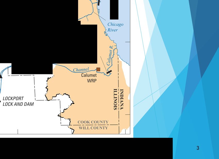
Lake Michigan Diversion and its monitoring

 ▪ Series of canals built from 1836 to 1922 connecting from Lake Michigan (Great
   Lakes Basin) to Illinois River (Mississippi River Basin).
 ▪ Primary canal is Chicago Sanitary and Ship Canal, completed in 1900.
 ▪ Reverses flow of Chicago River and diverts water from Lake Michigan.
 ▪ Diversion by State of Illinois from Great Lakes is limited by U.S. Supreme Court
   decree to a long-term mean of 3,200 cubic feet per second (ft3/s).
 ▪ U.S. Army Corps of Engineers is charged with monitoring the diversion: Lake
   Michigan Diversion Accounting (LMDA) program.

                                                                                      2
88° 00'                         87 ° 45'                              87 ° 30'

Chicago Sanitary and
                                                                                                                                                                                           I

Ship Canal and related
features of the
                                                                                  42 ° 00'
                                                                                                                                                                                LAKE
                                                                                                                                                                              MICHIGAN

Chicago Area
Waterway System                                                                                                                                 ■
                                                                                                                                                  Stickney
                                                                                                                                                  WRP      \
                                                                                                                                                           cciti(\
                                                                                                                                                                                  South
                                                                                                                                                                                  Branch

                                                                                                                                          ���         ·.)
                                                                                  41 ° 45'

                                                                                                                                                J/LOCK AND DAM
                                                                                                                                   .,��                              O'BRIEN
                                                                                                                                S��\
                                                                                                                          ---- Calumet /,r,.,
                                                                                                                r __,.(l,v-o 05536890 . Sa g
                                                                                                                 cnic    'b

                                                                                                                                           (

     -
                                                                                                 05536995
                          EXPLANATION
                   [WRP, Water Reclamation Plant]
                Diverted Lake Michigan watershed
                Divide between Lake Michigan Basin and
                   Mississippi River Basin before Lake Michigan
                   diversion                                                      41 °30'
   0553699�     U.S. Geological Survey streamgage and identifier

  U.S. Geological Survey streamgages shown on the map are as follows:
  Chicago Sanitary and Ship Canal at Romeoville, Illinois (station 05536995),                Base from U.S. Geological Survey 1 :100,000-scale             0              5          10 MILES
  and Chicago Sanitary and Ship Canal near Lemont, Illinois (station 05536890).              digital data, 2014, Albers Equal-Area Conic projection
                                                                                                                   °       °
                                                                                             Standard parallels 33 and 45 , central meridian 89
                                                                                                                                                 °
                                                                                                                                                           o          5       10 KILOMETERS
                                                                                             North American Datum of 1927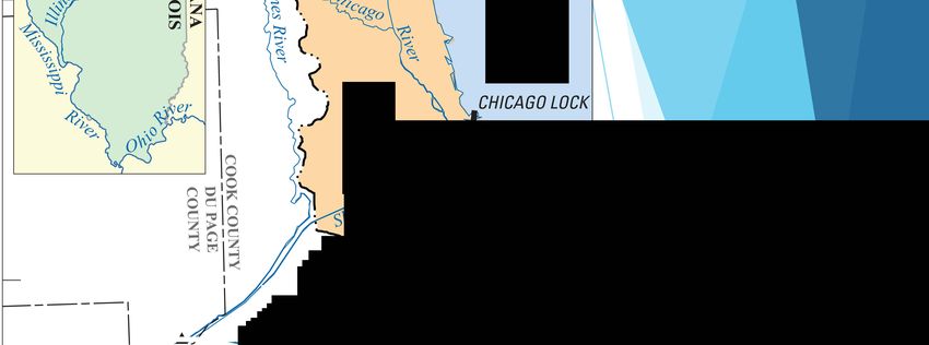
Streamgaging for LMDA and estimation of the
uncertainty of computed discharge based on it

▪ U.S. Geological Survey (USGS) has operated one or more streamgages on the
  Chicago Sanitary and Ship Canal for the LMDA program since 1984.
▪ Current primary streamgage for LMDA is “Chicago Sanitary and Ship Canal
  near Lemont, Illinois”, USGS streamgage 05536890 (hereafter, the “Lemont
  streamgage”) .
▪ Prior LMDA discharge computation uncertainty work focused on a statistical
  approach, using properties of the index-velocity rating regression (Over and
  others, 2004; Duncker and others, 2006).
▪ Present (2021) effort continues that approach but also investigates
  incorporation of measurement uncertainty in stage, index velocity, and
  discharge.                                                                     4

Lemont streamgage

   Gage house and instrumentation      On the Chicago Sanitary and Ship Canal looking
    (Modified from Jackson (2018).   downstream (southwest) toward streamgage during
    Photograph by Clayton Bosch,               installation of uplooking ADCP
      U.S. Geological Survey.)       (photograph by James Duncker, U.S. Geological Survey.)
                                                                                              5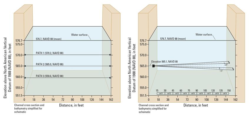
Lemont streamgage
Plan view                                                                                                Uplooking acoustic
                                                                                                          Doppler current
                                                                                                              profiler

                                                                    Gage           Buried                                                            162 feet
                                                                    house                cables
                       N

                                                    Sloughed bank
                                                                                                    o
                                                                                             44.5
               EXPLANATION                                                                                   o
                                                                                                        20
    Elevation, in feet above North American
                                                                                                                                 Acoustic Doppler velocity meter
       Vertical Datum of 1988
                                                                                                                                 (ADVM; black lines are the centers

                                                                                       AVM
                                                                       Cross-channel                                             of each beam and red lines show
                 High: 568.14                                                 cables                                             approximate width of each beam)
                                                                                                                   Discharge measurement cross section
                 Low: 548.98                      Flow
                                                                                                                 Centerline of ADVM (perpendicular to channel)

                                                                                                        AVM: Acoustic velocity meter

                                              Figure is from Jackson and others (2012)
                                                                                                                                                                      6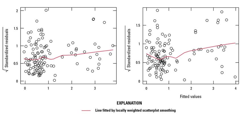
Instrumentation
 1. Stage: Paroscientific PS-2 pressure transducer with nitrogen tank and Conoflow gas-
    purge bubbler system.
 2. AVM: 3-path Accusonic O.R.E. 7510 GS temperature-compensated time of travel
    velocity meter.
     a.   Path length: 234.8 feet (ft), angle: 44.5 degrees
     b.   Path stages: 18.4, 13.2, 7.8 ft
 3. Horizontal ADVM (primary index velocity): TRDI Channel Master, 600 kHz
     a.   9 cells at 5 meters (16 ft) per cell beginning 2 meters (7 ft) from right (north) bank.
     b.   Stage: 13.2 ft.
 4. Discharge: ADCP (TRDI Rio Grande) measurements from moving boat (using tagline).
 5. Uplooking ADCP: not used in this study.

                                                                                                    7
Deployment schematics of the AVM (left) and the ADVM
(right) at the Lemont streamgage

         Schematic of the channel cross-section showing                 Schematic of the channel cross-section showing
         the three paths of the AVM (looking upstream).                 the ADVM beams (looking upstream).

                                        Figures are from Jackson and others (2012).                                      8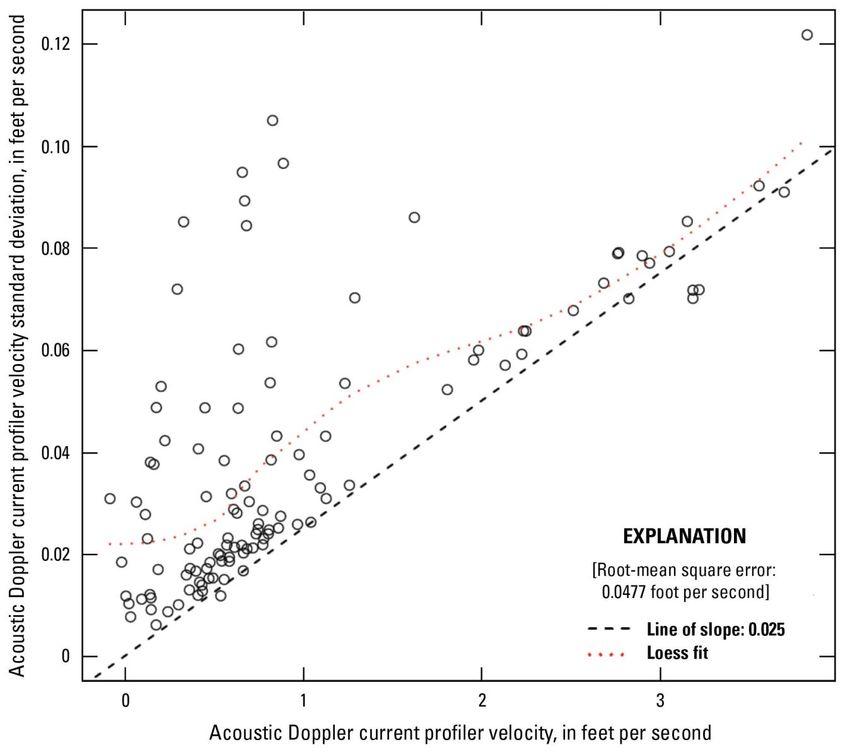
Approach to Uncertainty Estimation

Four steps:
1. Estimation of measurement uncertainty at continuous sensors by first-order
   second moment (FOSM) method using a type B approach: AVM, ADVM, and
   stage.
2. Estimation of uncertainty of ADCP calibration measurements (Qms).
3. Determination of AVM and ADVM-based index-velocity ratings (IVRs).
4. Computation of discharge and its uncertainty using IVRs.

                                                                                9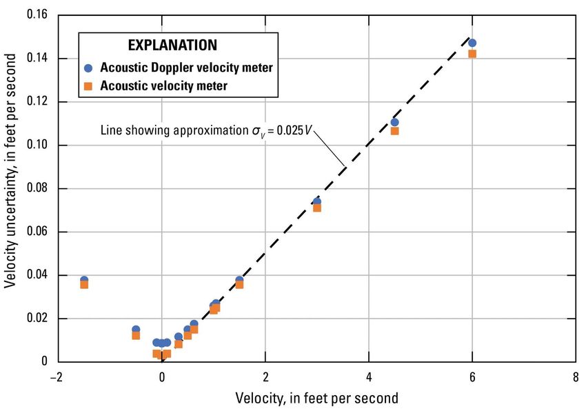
Discharge measurement dataset
•   155 ADCP discharge measurements (Qms) and corresponding ADVM and AVM velocities
    were processed using QRev (Mueller, 2016) for this study (Prater and others, 2021). Of
    these,
     o 140 have corresponding AVM velocities.
     o 130 have corresponding ADVM velocities.
     o 115 have both.
•   Dataset properties include:
     o Date range: Jan. 12, 2005, to Oct. 23, 2013.
     o Measured discharge, range: −344 to 16,794 ft3/s; median: 2,605 ft3/s
     o Duration of measurement, range: 162 to 3,563 seconds; median: 831 seconds.
     o Number of transects, range: 1 to 18; median: 4.

                                                                                             10
Step 1: Estimation of measurement uncertainty
at continuous sensors
▪ Sensors: AVM, ADVM, pressure transducer
▪ General approach: “type B,” with computations by first-order
second moment (FOSM) method.
▪ Software: QMSys (http://www.qsyst.com), implements FOSM
and Monte Carlo methods.
11Error Propagation by the First-order Second Moment
(FOSM) Method
Uncertainty in FOSM method is computed as the variance , the 2nd moment, of Y, which is a
function of some X variables:
Using properties of variance and a Taylor series (first-order) expansion, variance of Y, is
approximately:
If X variables are independent, then:
For example, for Q = AV, one gets:
(adapted from Duncker and others, 2006).
12AVM uncertainty – Data reduction equation (DRE)
where:
VL = “line velocity,” velocity along acoustic path, used as index velocity,
B = acoustic path length,
A = angle between acoustic path and velocity, and
TCD, TDC = travel times of acoustic signal between transmitter and receiver and back.
At the Lemont streamgage, the line velocities from three acoustic paths are averaged (with
weighting when one or more is missing) to obtain a composite mean AVM velocity (Jackson
and others, 2012).
Note that the DRE is nonlinear in all quantities except the acoustic path length B.
13AVM uncertainties: Expanded DRE as entered
into QMSys
Part of QMSys input window
14Elemental uncertainties for AVM velocity at low flow*
Name Notation Error category Absolute Contribution to total
uncertainty uncertainty (ft/s)**
Acoustic path length SI1 Site and installation 0.02% 8e-7
Changes in spatial flow distribution SI2 Site and installation 1% 0.001258
Acoustic path angle SI3 Site and installation 0.17% 0.000036
Travel time I1 Instrument 30 nsec 0.001056
Instrument resolution I2 Instrument 0.001 ft/s 0.000121
Sampling frequency OC1 Operation - Configuration 1% 0.001258
Sampling time OC2 Operation – Configuration 0 0
Time synchronization OC3 Operation – Configuration Not applicable*** 0
Operational issues OO1 Operation – Operator 0 0
Wind-induced shear OM1 Operation – Measurement 1% 0.001258
Acoustic path deflection OM2 Operation – Measurement 1% of B, A 0.001992
Temporary changes in flow distribution OM3 Operation – Measurement 1% 0.001258
Total 0.00824 (2.56% of V)
*Low flow selected as discharge = 1,300 ft3/s; velocity (V) = 0.322 ft/s; stage = 24.92 ft.
**Computed as the square root of the variance associated with this component. 15
***Not applicable to AVM velocity by itself but when used in rating curve development.AVM uncertainties:
FOSM estimates Absolute and relative
from QMSys contributions of elemental
uncertainties
Comparison of
distributions of FOSM
and Monte Carlo results
16ADVM uncertainty estimation: DREs
Basic data reduction equation (DRE):
where:
Vi = Velocity along the acoustic path
Fd = Doppler shift of received frequency
Fs = Transducer transmit frequency
C = Speed of sound
Expanded DRE as used for uncertainty estimation in QMSys:
17Elemental uncertainties for ADVM velocity at low flow*
Name Notation Error category Absolute uncertainty Contribution to total
uncertainty (ft/s)**
Beam orientation SI1 Site and installation 0 0
Changes in spatial flow distribution SI2 Site and installation 2% 0.003501
Accuracy I1 Instrument 2 mm/s 0.003634
Resolution I2 Instrument 1 mm/s 0.000908
Factory settings I3 Instrument 1 mm/s 0.000908
Analytical methods I4 Instrument 1 mm/s 0.000908
Measurement volume setting OC1 Operation - Configuration 0 0
Sampling frequency, sampling time OC2, OC3 Operation – Configuration 0, 0 0, 0
Data logger, compass OC4, OC5 Operation – Configuration 0, 0 0, 0
Salinity input OO1 Operation – Operator 0.463% 0.000187
Wind-induced shear OM1 Operation – Measurement 1% 0.000875
Acoustic path deflection OM2 Operation – Measurement Not determined 0
Temporary changes in flow distribution OM3 Operation – Measurement 1% 0.000875
Total 0.0118 (3.66% of V)
*Low flow selected as discharge = 1,300 ft3/s; velocity (V) = 0.322 ft/s; stage = 24.92 ft.
**Computed as the square root of the variance associated with this component. 18Predicted AVM and ADVM velocity uncertainties Notice: ▪ Strong dependence of total velocity uncertainty sv on velocity V : sv ≈ 0.025V. ▪ sAVM_V < sADVM_V esp. for small V ▪ At V=0, sAVM_V = 0.0031 ft/s and sADVM_V = 0.0087 ft/s. ▪ Per current DREs, s−V = sV (mirrored around V = 0). sAVM_V : total uncertainty of AVM velocity. sADVM_V : total uncertainty of ADVM velocity. Note: The ADVM results shown here do not consider the effect of salinity. 19
Water-level (stage) uncertainty estimation: DRE

                           Part of QMSys input window

                                                        20
Elemental uncertainties for water level (stage)
Name Notation Error category Absolute uncertainty Contribution to total
uncertainty (ft)*
Datum errors SI1 Site and installation 0 0
Local disturbances SI2 Site and installation 0.02 ft 0.014728
Accuracy I1 Instrument 0.02% 0.001325
Resolution I2 Instrument 0.01 ft 0.003682
Calibration, Data transmission I3, I4 Instrument 0, 0 0, 0
Timing, Data logger I5, I6 Instrument 0, 0 0, 0
Gage offset OC1 Operation - Configuration 0.01 ft 0.003682
Recorder, Data retrieval OC2, OC3 Operation – Configuration 0, 0 0, 0
Periodic stage correction OC4 Operation – Configuration 0.01 ft 0.003682
Operational issues OO1 Operation - Operator 0 0
Hydraulically induced OM1 Operation - Measurement 0 0
Temperature effects OM2 Operation – Measurement 0 0
Temporary flow disturbances OM3 Operation - Measurement 0 0
Total 0.0271 ft
*Computed as the square root of the variance associated with this component.
21Step 2: Estimation of discharge (ADCP) uncertainties
▪ No generally accepted detailed method of ADCP uncertainty estimation yet exists.
▪ Used approximate estimates from QRev (Mueller, 2016).
▪ QRev uncertainty estimates consider the following:
1. Random uncertainty: coefficient of variation (CV) = standard deviation / mean of transect
discharges
2. Invalid data uncertainty
3. Top/bottom extrapolation uncertainties
4. Edge estimation uncertainty
5. Moving bed test uncertainty (when bottom tracking used)
6. Systematic uncertainty: 1.5 percent (one-standard deviation estimate)
Note: Any such single Qm uncertainty estimate does not address correlation among Qms,
which would affect the index-velocity rating and its uncertainty.
22Results of QRev estimation of ADCP uncertainties
Uncertainty statistics for all 155 measurements
Computation (in terms of standard uncertainties in considered in this study, expressed as standard
Uncertainty source uncertainties in percent
percent)
Minimum Median Maximum
Random uncertainty Proportional to the CV of the transect discharges 0.2 3.3 243
10 percent of the percentage discharge for invalid cells
Invalid data uncertainty 0 0 3.75
and ensembles
Edge uncertainty 15 percent of the percentage discharge in the edges 0.45 1.75 7.9
Top/bottom extrapolation Based on variation among results of different
0.05 0.2 9.45
uncertainty extrapolation methods
If bottom track used: 0.5 if no moving bed, 0.75 if moving
Moving-bed test uncertainty bed is present, 1.5 percent if moving-bed test not 0 1.5 1.5
performed; otherwise 0.
Systematic uncertainty Fixed at 1.5 percent 1.5 1.5 1.5
Total uncertainty 2.2 4.3 243
23Estimated ADCP
uncertainties
▪ Plot shows common Qms with ADCP V s
computed using ADVM stage-area rating.
▪ Minimum “base” uncertainty estimate of
~0.025V (~same as ADVM, AVM):
Primary error sources: systematic, edges, moving
bed.
▪ High “outliers”:
▪ common for V < 2 ft/s
▪ Primary sources: random (CV), extrapolation.
▪ Root-Mean Square Error (RMSE) of ADCP V s,
RMSE(VADCP) = 0.0477 ft/s
▪ RMSE(VADVM) = 0.0356 ft/s
▪ RMSE(VAVM) = 0.0345 ft/s
24Step 3: Determination of Index-Velocity
Ratings
25Index-velocity ratings
• Per standard USGS practice (Levesque and Oberg, 2012), index-velocity ratings (IVRs) are
developed by fitting a linear regression line with velocities from discharge measurements,
VQm = Qm /Areaindex,
where
Qm is a discharge measurement and
Areaindex is the cross-sectional area from the stage-area rating associated with the index-
velocity meter,
as the predictand (y-axis variable) to velocities from the index-velocity meter, Vindex.
• A straight-line fit, that is,
VQm = a + bVindex
is used unless a pattern such as curvature is seen in the regression residuals.
• Each of the two index-velocity meters at the Lemont streamgage considered in this study has its
own stage-area rating curve and its own set of IVRs.
• In this study, only straight-line fits were deemed necessary.
26Stage-Area ratings
• At the Lemont streamgage, there are two index-velocity meters; each has a
stage-area rating curve to be used for determining Areaindex:
AVM Areaindex = 179.403×Stage − 638.05
ADVM Areaindex = 164.6766×Stage − 71.0209.
• The differences between these stage-area rating curves arise from the AVM
paths traversing the part of the measurement site that includes the sloughed
bank, whereas the ADVM is located upstream (west) from this part of the channel
(see measurement site plan, slide 6).
27Assumptions of ordinary least squares (OLS) regression and
their implications
Table taken
from Helsel
and others
(2020), p. 228.
[y, response variable; x, predictor variable]
28Empirical distributions of ADVM and AVM velocity data
Data type Number of Mean Mini- 1% 10% Median 90% 99% Maxi-
data points mum quantile quantile quantile quantile mum
ADVM velocities used for IVRs, ft/s 130 0.978 −0.036 0.034 0.183 0.68 2.78 3.69 3.88
ADVM prediction velocities, ft/s 464,077 0.685 −0.28 0.061 0.269 0.57 1.19 3.00 4.58
AVM velocities used for IVRs, ft/s 140 0.947 −0.037 −0.003 0.195 0.62 2.74 3.60 4.03
AVM prediction velocities, ft/s 509,996 0.719 −0.390 0.030 0.280 0.61 1.23 3.11 4.80
29Regression methods considered
Are errors on the x
Are errors Is correlation of ADCP
Regression method (index velocity) Software packages used
specified? errors considered?
axis considered?
Ordinary least squares (OLS) No No No R (lm function)
Weighted least squares (WLS) No No No R (lm function)
Weighted least squares (WLS) Yes No No R (lm) and TS28037a
Gauss-Markov regression (GMR) (also called
Yes No Yesb TS28037
generalized least squares: GLS)
Generalized distance regression (GDR) (also called
Yes Yes No TS28037
errors-in-variables regression: EIV)
Generalized Gauss-Markov regression (GGMR)c Yes Yes Yes TS28037
aTS28037: Software to Support ISO/TS 28037:2010(E) (National Physical Laboratory, 2010).
bTwo assumptions on correlations of the ADCP errors were tested: (1) that those measurements made in immediate succession have
correlations of 0.5; and (2) that all the ADCP measurements are correlated with correlation = 0.1.
cBasic results with GGMR regression were computed but are not presented here to avoid unnecessary complexity.
30Regression software used for fitting IVRs
Two packages:
1. Specified errors: MATLAB software built to implement ISO/TS 28037 (National Physical Laboratory,
2010).
2. Unspecified errors: General linear regression by lm function (R Core Team, 2019).
RStudio window
31Chi-squared (C 2) tests of regression model fits
• Without specified measurement uncertainties, one typically uses a variety of diagnostics that mostly focus
on the properties of the residuals (Helsel and others, 2020, chapter 9).
• With specified measurement uncertainties, the C 2 test (Press and others, 1992, p. 653–655), can be applied
to test the model fit as follows:
o If the specified measurement uncertainties are correct (that is, they are Gaussian with specified
variances) and the (linear) model is appropriate, then
SSRnorm = sum of squared regression residuals normalized by uncertainties has a C 2 distribution
with n−p degrees of freedom, denoted C 2n−p ,
where
n = number of data points used and
p = number of parameters fitted (here, 2).
o C 2n−p has mean n−p and variance 2(n−p) so a value of SSRnorm near n−p is expected.
o If the test fails, meaning p = Prob(C 2n−p > SSRnorm) < a, for some selected significance level aComparison of OLS ADVM and AVM Index Velocity
Ratings (on common Qms)
SE(AVM IVR) = 0.104 ft/s > SE(ADVM IVR) = 0.056 ft/s
4
4
(acoustic Doppler current profiler velocity,
(acoustic Doppler current profiler velocity,
Discharge measurement per area
Discharge measurement per area
3
3
in feet per second)
in feet per second)
2 2
1 Coefficients Coefficients
1
Intercept, in feet per second: −0.01167 Intercept, in feet per second: 0.03083
Slope: 0.97427 Slope: 0.97896
Intercept standard error, in feet per second: 0.00756 Intercept standard error, in feet per second: 0.01378
Slope standard error: 0.00537 Slope standard error: 0.00951
Correlation of coefficients: −0.72352 Correlation of coefficients: −0.70901
0 Standard error, in feet per second: 0.05598 0 Standard error, in feet per second: 0.1042
0 1 2 3 4 0 1 2 3 4
Acoustic Doppler velocity meter index velocity, Acoustic velocity meter index velocity, in feet per second
in feet per second
33Distributions of OLS IVR residuals (common Qms)
ADVM AVM
Gaussian quantile-quantile plot Gaussian quantile-quantile plot
▪ Confirms AVM residuals > ADVM residuals
▪ Confirms presence of (non-Gaussian) outliers 34Heteroscedasticity of OLS IVR residuals (common Qms)
ADVM AVM
Scale-location plot Scale-location plot
Results of statistical tests of heteroscedasticity (ADVM and AVM, respectively):
1. Non-constant variance test (Helsel and others, 2020, p. 244): p = 0.006 and 0.00001.
2. Kendall’s tau correlation with fitted values (Helsel and others, 2020, section 8.4):
tau = 0.119 and 0.099; two-sided p = 0.060 and 0.117.
35AVM vs. ADVM
OLS IVR
residuals
Correlation of residuals is positive
but not especially large, indicating
ADCP errors are on the same
order of magnitude as ADVM and
AVM.
36Intercept, slope, and C 2 test statistics for ADVM-based IVRs
for selected regression methods and error specifications
Are Are IV
Correlation Prob(C 2n−p >
Regression errors errors Correlation of Intercept Intercept
Slope Slope SE (Intercept, SSRnorm SSRnorm) (n−p
method speci- consi- ADCP errors (ft/s) SE (ft/s)
Slope) = 128)
fied? dered?
OLS No No None −0.0071 0.9740 0.0073 0.0054 −0.727 N/A N/A
WLS Yes No None −0.0336 1.0017 0.0028 0.0049 −0.747 743.3 < 1e−16
WLS aYes ×2 No None −0.0336 1.0017 0.0056 0.0097 −0.747 185.8 0.00064
GMR (GLS) Yes No bsel.corr. = 0.5 −0.0383 1.0066 0.0032 0.0062 −0.753 932.6 < 1e−16
GMR (GLS) aYes ×2 No bsel.corr. = 0.5 −0.0383 1.0066 0.0064 0.0125 −0.753 233.2 3.9e−8
GMR (GLS) Yes No ccorr. = 0.1 −0.0359 0.9937 0.0029 0.0061 −0.246 822.0 < 1e−16
GMR (GLS) aYes ×2 No ccorr. = 0.1 −0.0359 0.9937 0.0058 0.0123 −0.246 205.5 1.6e−5
GDR (EIV) Yes Yes None −0.0349 1.0094 0.00395 0.00668 −0.754 366.6 < 1e−16
GDR (EIV) aYes ×2 Yes None −0.0349 1.0094 0.00790 0.01336 −0.754 91.7 0.99
[IV, index velocity]
a”× 2” here means that the estimated standard errors, both ADCP and IV, were multiplied by 2.
bErrors of ADCP (y-axis) measurements in immediate succession were assigned correlations of 0.5.
cErrors of all ADCP (y-axis) measurements were assigned correlations of 0.1.
37Intercept, slope, and C 2 test statistics for AVM-based IVRs
for selected regression methods and error specifications
Are Are IV
Correlation Prob(C 2n−p >
Regression errors errors Correlation of Intercept Intercept
Slope Slope SE (Intercept, SSRnorm SSRnorm) (n−p
method speci- consi- ADCP errors (ft/s) SE (ft/s)
Slope) = 138)
fied? dered?
OLS No No None 0.0400 0.9768 0.0123 0.0092 −0.707 N/A N/A
WLS Yes No None 0.0106 0.9899 0.0027 0.0048 −0.733 1594 < 1e−16
WLS aYes ×3 No None 0.0106 0.9899 0.0081 0.0143 −0.733 177.2 0.014
GMR (GLS) Yes No bsel.corr. = 0.5 0.0014 0.9977 0.0031 0.0063 −0.746 1748 < 1e−16
GMR (GLS) aYes ×3 No bsel.corr. = 0.5 0.0014 0.9977 0.0093 0.0188 −0.746 194.2 0.0012
GMR (GLS) Yes No ccorr. = 0.1 0.00076 0.9616 0.0029 0.0060 −0.175 1721 < 1e−16
GMR (GLS) aYes ×3 No ccorr. = 0.1 0.00076 0.9616 0.0088 0.0181 −0.175 191.2 0.0019
GDR (EIV) Yes Yes None 0.0069 1.0057 0.0032 0.0061 −0.723 1168 < 1e−16
GDR (EIV) aYes ×3 Yes None 0.0069 1.0057 0.0095 0.0182 −0.723 129.8 0.68
a”× 3” here means that the estimated standard errors, both ADCP and IV, were multiplied by 3.
bErrors of ADCP (y-axis) measurements in immediate succession were assigned correlations of 0.5.
cErrors of all ADCP (y-axis) measurements were assigned correlations of 0.1.
38Prediction statistics for ADVM-based IVRs for selected
regression methods and error specifications
Mean bias Variance ratio
Are errors Are IV errors Correlation of ADCP Mean SE of
Regression method (predicted – (predicted to
specified? considered? errors prediction (ft/s)
observed) (ft/s) observed)
OLS No No None 0.00000 0.0572 0.996
WLS Yes No None 0.00058 0.0627 1.054
WLS aYes ×2 No None 0.00058 0.0627 1.054
GMR (GLS) Yes No bsel.corr. = 0.5 0.00071 0.0649 1.064
GMR (GLS) aYes ×2 No bsel.corr. = 0.5 0.00071 0.0649 1.064
GMR (GLS) Yes No ccorr. = 0.1 −0.00957 0.0608 1.037
GMR (GLS) aYes ×2 No ccorr. = 0.1 −0.00957 0.0608 1.037
GDR (EIV) Yes Yes None 0.00680 0.0664 1.070
GDR (EIV) aYes ×2 Yes None 0.00680 0.0664 1.070
a”× 2” here means that the estimated standard errors, both ADCP and IV, were multiplied by 2.
bErrors of ADCP (y-axis) measurements in immediate succession were assigned correlations of 0.5.
cErrors of all ADCP (y-axis) measurements were assigned correlations of 0.1.
39Prediction statistics for AVM-based IVRs for selected
regression methods and error specifications
Mean bias Variance ratio
Are errors Are IV errors Correlation of Mean SE of
Regression method (predicted – (predicted to
specified? considered? ADCP errors prediction (ft/s)
observed) (ft/s) observed)
OLS No No None 0.00000 0.1032 0.988
WLS Yes No None −0.0169 0.1053 1.015
WLS aYes ×3 No None −0.0169 0.1053 1.015
GMR (GLS) Yes No bsel.corr. = 0.5 −0.0188 0.1068 1.031
GMR (GLS) aYes ×3 No bsel.corr. = 0.5 −0.0188 0.1068 1.031
GMR (GLS) Yes No ccorr. = 0.1 −0.0536 0.1173 0.957
GMR (GLS) aYes ×3 No ccorr. = 0.1 −0.0536 0.1173 0.957
GDR (EIV) Yes Yes None −0.0057 0.1070 1.047
GDR (EIV) aYes ×3 Yes None −0.0057 0.1070 1.047
a”× 3” here means that the estimated standard errors, both ADCP and IV, were multiplied by 3.
bErrors of ADCP (y-axis) measurements in immediate succession were assigned correlations of 0.5.
cErrors of all ADCP (y-axis) measurements were assigned correlations of 0.1.
40Step 4: Computed Discharge Uncertainty
41Computation of discharge with an index-velocity rating
With an IVR VQm(Vindex) and a stage-area rating Areaindex(h), where h is stage, and
continuous measurements of velocity Vindex(t) and stage h(t), where t is time, discharge at
time t, Q(t), is computed by multiplying the rated velocity by the rated area given, that is:
Q(t) = VQm(Vindex(t)) × Areaindex(h(t)).
Because here VQm(Vindex) = a + b*Vindex, where a is intercept and b is the slope of the IVR,
the discharge computation relation can be written more specifically as:
Q(t) = [a + b*Vindex(t)] × Areaindex(h(t)).
42Sources of uncertainty in discharge computed with index-
velocity ratings
Because the computed discharge is a product of rated velocity and rated area, likewise its uncertainty
arises from those factors.
From the rated velocity, which is more properly written as
VQm = a + bVindex + e,
where e is the IVR fitting error, there are two components:
1. The uncertainty of the IVR parameters a and b, which are distributed as a joint Gaussian distribution
with mean vector [a,b] and covariance matrix parameterized by their individual SEs and their
correlation (see slides 37 and 38 for values).
2. The uncertainty arising from e, which may or may not be correlated in time, and whose uncertainty
magnitude is computed from the regression residuals.
The error in Areaindex(h(t)) is neglected here because, according to the argument of Duncker and others
(2006, p. 28), the error in the stage-area rating is eliminated because the same stage-area rating is used in
the fitting of the IVR and the computation of discharge.
43Effect of time scale of averaging on computed discharge
uncertainty USGS 05536995, Chicago Ship and Sanitary Canal at Romeoville, Illinois
At this similar streamgage, which
10−1
was also on the Chicago Sanitary EXPLANATION
and Ship Canal and was the Uncertainty sources
Discharge uncertainty as coefficient of variation
Index-velocity rating parameters
primary measurement location 10−2
Area estimation
for LMDA discharge Index-velocity rating standard error
measurements before it was 10−3
Total
moved about 6 miles upstream to
Lemont, and where discharge 10−4
was computed with an IVR based
on AVM velocities, at long time 10−5
scales (monthly to annual), IVR
regression parameter uncertainty
10−6
was determined to dominate
computed discharge uncertainty
(Over and others, 2004). 10−7
10−3 10−2 10−1 100 101 102 103
Averaging time scale, in days
Figure is adapted from presentation by Over and others (2004).
44Computation of discharge and its uncertainty by
Monte Carlo simulation
• For each index-velocity meter, the uncertainty in the IVR parameters a and b was simulated by
sampling a vector [a,b] from their joint Gaussian distribution 100 times.
• When using the OLS IVR, the IVR error term e was also simulated as an independent Gaussian time
series e(t) with zero mean and standard deviations (stdevs) from the SEs of the OLS IVR regressions
(ADVM: 0.0572 ft/s; AVM: 0.1032 ft/s).
• For each sample of [a,b], discharge Q(t) was computed by the standard method for streamgages with
IVRs (slide 40) at a 10-minute time step.
• In each day, if at least half the 10-minute Q(t) values were available, those Q(t) values were averaged to
compute a daily mean.
o Otherwise, 10-minute Q(t) values from the other index-velocity meter were used if at least half of
those were available.
▪ Otherwise, the day was left as missing.
• Finally, the daily values were averaged to obtain water-year-annual mean Q(t) values.
• AVM data were available for most of WYs 2006–15 and ADVM data for most of WYs 2008–16, and
therefore those years were simulated for each respective index-velocity meter. 45Uncertainty statistics for annual mean (water years 2008–16) computed
discharge for ADVM-based IVRs for selected regression methods and
error specifications
Mean of annual
Regression Are errors Are IV errors Correlation of Mean of annual Mean of daily CVs ±
means ±
method specified? considered? ADCP errors stdevs (ft3/s) stdev(CVs)
stdev(mean) (ft3/s)
OLS No No None 2,660 ± 2 21.2 0.595 ± 0.0007
WLS Yes No None 2,625 ± 1 9.5 0.621 ± 0.0003
WLS aYes ×2 No None 2,625 ± 2 18.1 0.620 ± 0.0005
GMR (GLS) Yes No bsel. corr. = 0.5 2,622 ± 1 12.2 0.625 ± 0.0003
GMR (GLS) aYes ×2 No bsel. corr. = 0.5 2,619 ± 2 18.0 0.626 ± 0.0006
GMR (GLS) Yes No ccorr. = 0.1 2,593 ± 2 19.5 0.623 ± 0.0003
GMR (GLS) aYes ×2 No ccorr. = 0.1 2,596 ± 3 33.4 0.623 ± 0.0006
GDR (EIV) Yes Yes None 2,638 ± 1 12.9 0.621 ± 0.0003
GDR (EIV) aYes ×2 Yes None 2,640 ± 2 22.2 0.623 ± 0.0008
a”× 2” here means that the estimated standard errors, both ADCP and IV, were multiplied by 2.
bErrors of ADCP (y-axis) measurements in immediate succession were assigned correlations of 0.5.
cErrors of all ADCP (y-axis) measurements were assigned correlations of 0.1.
Computed at a 10-minute time step with 100 Monte Carlo samples. On average 6.3 days per year were filled with
AVM-based computed discharge, when available; on average 1 day per year remains missing. 46OLS regression parameter uncertainty-based Monte Carlo results for
computed discharge using ADVM velocities
47Uncertainty statistics for annual mean (water years 2006–15) computed
discharge for AVM-based IVRs for selected regression methods and error
specifications
Mean of annual
Are errors Are IV errors Correlation of Mean of annual Mean of daily CVs ±
Regression method means ±
specified? considered? ADCP errors stdevs (ft3/s) stdev(CVs)
stdev(mean) (ft3/s)
OLS No No None 2,834 ± 3 34.5 0.545 ± 0.0009
WLS Yes No None 2,756 ± 1 8.9 0.568 ± 0.0002
WLS aYes ×3 No None 2,755 ± 3 28.7 0.566 ± 0.0006
GMR (GLS) Yes No bsel. corr. = 0.5 2,742 ± 1 12.1 0.575 ± 0.0002
GMR (GLS) aYes ×3 No bsel. corr. = 0.5 2,750 ± 3 33.4 0.572 ± 0.0007
GMR (GLS) Yes No ccorr. = 0.1 2,643 ± 2 18.2 0.575 ± 0.0002
GMR (GLS) aYes ×3 No ccorr. = 0.1 2,646 ± 6 57.6 0.575 ± 0.0007
GDR (EIV) Yes Yes None 2,784 ± 1 11.9 0.570 ± 0.0003
GDR (EIV) aYes ×3 Yes None 2,786 ± 3 32.2 0.571 ± 0.0008
a”× 3” here means that the estimated standard errors, both ADCP and IV, were multiplied by 3.
bErrors of ADCP (y-axis) measurements in immediate succession were assigned correlations of 0.5.
cErrors of all ADCP (y-axis) measurements were assigned correlations of 0.1.
Computed at a 10-minute time step with 100 Monte Carlo samples. On average 9.1 days per year were filled with
48
ADVM-based computed discharge, when available; on average 1.2 days per year remains unfilled.OLS regression parameter uncertainty-based Monte Carlo results for
computed discharge using AVM velocities
49Summary I: Predicted measurement uncertainties
• Type B (non-empirical, scientific judgment-based) estimates for ADVM and AVM velocities and
stage at the Lemont streamgage were developed using FOSM and checked using Monte Carlo
simulation.
• Elemental uncertainties were taken as Gaussian, and predicted uncertainties were also Gaussian
to a high degree of approximation.
• ADVM and AVM velocities were predicted to be similar and about 2.5 percent of velocity except
near zero velocity, where AVM uncertainty was predicted as about 0.003 ft/s and ADVM
uncertainty as about 0.009 ft/s.
• Stage uncertainty was estimated to be about 0.027 ft, independent of water level.
• Measured discharge Qm uncertainty was estimated using QRev (Mueller, 2016), which is part
empirical and part judgment based.
• When converted to mean channel velocities, the predicted Qm uncertainties were estimated to be
larger than the AVM and ADVM uncertainties, being at least 2.5 percent of velocity, but often much
larger, especially for lower velocities.
50Summary II: Index-velocity ratings (IVRs) computed using
ordinary least squares (OLS) regression
• Used a database of 155 ADCP discharge – index velocity pairs:
o 155 total pairs, 140 with AVM velocity, 130 with ADVM velocity, 115 with both.
o Distribution of velocities in database agree with prediction velocities except at moderately high values.
• OLS-fitted IVRs were found to be linear with high coefficient of determination (R 2) values (at least 0.988).
• Properties of OLS residuals:
o Residual standard error of AVM regression (0.104 ft/s) were about twice that of ADVM (0.056).
o Distributions of both sets of residuals had fat, non-Gaussian tails.
o Both AVM and ADVM residuals showed modest growth with velocity.
o AVM and ADVM residuals from common measurements were modestly positively correlated, indicating
contributions from both index-velocity and ADCP errors.
• When repredicting fitting data, OLS predictions were unbiased, had the smallest prediction error, and
had only a small variance reduction effect.
51Summary III: Index-velocity ratings computed using
alternative regressions
• Alternative regression methods used allow:
o Variation in uncertainties of regression data on y axis or both x and y axes.
o Specification of measurement errors for which the predicted index-velocity and ADCP uncertainties were used.
• C 2 tests of residuals of alternative regressions indicate:
o predicted measurement uncertainties are too small.
o predicted measurement uncertainties need to be multiplied by about 2 (ADVM) or 3 (AVM).
52Summary IV: Computed discharge and its uncertainty
• Uncertainty sources other than uncertainty of IVR parameters assumed to be negligible at annual
time scale.
• Used Monte Carlo simulation.
• Water years 2008–16 (ADVM) and 2006–15 (AVM) predicted.
• Properties of computed discharge using OLS regression:
o Coefficients of variation (CVs) of 0.8 percent (ADVM) and 1.2 percent (AVM) of annual means.
o Largest mean discharges.
o Smallest variation of daily discharges.
• Properties of computed discharge using alternative regressions:
• Similar CVs as OLS only when specified uncertainties were increased by 2 or 3.
• Smaller mean discharges.
• Larger variation at daily time scale.
• Concluded OLS-based results should be reliable if not exact.
53Summary V: Final Remarks
• Results indicate need to revisit predicted measurement uncertainties (magnitude, velocity
dependence).
• Measurements with larger residuals could be examined individually regarding possible
causes.
• Improved methods of ADCP uncertainty estimation may be or may soon be available.
• Main weakness of OLS regression probably is correspondence of fitting and prediction
velocity distributions:
o Could be addressed by subsampling or additional measurements.
• Better inference of growth in residuals with velocity would help IVR regressions and
predicted measurement uncertainties.
54References Cited - 1
• Duncker, J.J., Over, T.M., and Gonzalez, J.A., 2006, Computation and error analysis of discharge for the Lake Michigan
Diversion Project in Illinois—1997–99 water years: U.S. Geological Survey Scientific Investigations Report 2006–5018, 70
p., accessed December 2016 at https://doi.org/10.3133/sir20065018.
• Helsel, D.R., Hirsch, R.M., Ryberg, K.R., Archfield, S.A., and Gilroy, E.J., 2020, Statistical methods in water resources:
U.S. Geological Survey Techniques and Methods, book 4, chap. A3, 458 p. [Also available at
https://doi.org/10.3133/tm4A3.]
• Jackson, P.R., 2018, Characterizing variability in vertical profiles of streamwise velocity and implications for
streamgaging practices in the Chicago Sanitary and Ship Canal near Lemont, Illinois, January 2014 to July 2017: U.S.
Geological Survey Scientific Investigations Report 2018–5128, 73 p., accessed November 2018 at
https://doi.org/10.3133/sir20185128.
• Jackson, P.R., Johnson, K.K., and Duncker, J.J., 2012, Comparison of index velocity measurements made with a
horizontal acoustic Doppler current profiler and a three-path acoustic velocity meter for computation of discharge in
the Chicago Sanitary and Ship Canal near Lemont, Illinois: U.S. Geological Survey Scientific Investigations Report 2011–
5205, 42 p., accessed September 2013 at https://doi.org/10.3133/sir20115205.
• Levesque, V.A., and Oberg, K.A., 2012, Computing discharge using the index velocity method: U.S. Geological Survey
Techniques and Methods, book 3, chap. A23, 148 p., accessed May 2015 at https://doi.org/10.3133/tm3A23.
55References Cited - 2
• Mueller, D.S., 2016, QRev—Software for computation and quality assurance of acoustic Doppler current profiler
moving-boat streamflow measurements—Technical manual for version 2.8: U.S. Geological Survey Open-File Report
2016–1068, 79 p., accessed October 2020 at https://doi.org/10.3133/ofr20161068.
• National Physical Laboratory, 2010, Software to support ISO/TS 28037:2010(E): National Physical Laboratory software
release, accessed December 14, 2016, at https://www.npl.co.uk/resources/software/iso-ts-28037-2010e.
• Over, T.M., Duncker, J.J., and Gonzalez-Castro, J.A., 2004, Comparison of estimates of uncertainty of discharge at
U.S. Geological Survey index-velocity gages on the Chicago Sanitary and Ship Canal, Illinois, in Sehlke, G., Hayes,
D.F., and Stevens, D.K., eds., Critical Transactions in Water and Environmental Resources Management—
Proceedings of the 2004 World Water and Environmental Resources Congress, Salt Lake City, Utah, June 27–July 1,
2004 [Conference paper]: Reston, Va., American Society of Civil Engineers, p. 2342–2352. [Also available at
https://doi.org/10.1061/40737(2004)288.]
• Prater, C.D., LeRoy, J.Z., Engel, F.L., and Johnson, K.K., 2021, Discharge measurements at U.S. Geological Survey
streamgage 05536890 Chicago Sanitary and Ship Canal near Lemont, Illinois, 2005-2013: U.S. Geological Survey data
release, https://doi.org/10.5066/F7X63K41.
• Press, W.H., Teukolsky, S.A., Vetterling, W.T., and Flannery, B.P., 1992, Numerical recipes in Fortran 77—The art of
scientific computing (2d ed.): New York, Cambridge University Press, 973 p.
• R Core Team, 2019, R—A language and environment for statistical computing, version 4.0.4 (Rd): R Foundation for
Statistical Computing software release, accessed February 25, 2021, at https://www.R-project.org/.
56You can also read