A General Optimization-based Framework for Global Pose Estimation with Multiple Sensors
←
→
Page content transcription
If your browser does not render page correctly, please read the page content below
A General Optimization-based Framework for Global
                                                                Pose Estimation with Multiple Sensors
                                                                             Tong Qin, Shaozu Cao, Jie Pan, and Shaojie Shen

                                            Abstract— Accurate state estimation is a fundamental prob-
                                         lem for autonomous robots. To achieve locally accurate and
                                         globally drift-free state estimation, multiple sensors with com-
                                         plementary properties are usually fused together. Local sensors
                                         (camera, IMU, LiDAR, etc) provide precise pose within a small
arXiv:1901.03642v1 [cs.CV] 11 Jan 2019

                                         region, while global sensors (GPS, magnetometer, barometer,
                                         etc) supply noisy but globally drift-free localization in a large-
                                         scale environment. In this paper, we propose a sensor fusion
                                         framework to fuse local states with global sensors, which
                                         achieves locally accurate and globally drift-free pose estimation.
                                         Local estimations, produced by existing VO/VIO approaches,
                                         are fused with global sensors in a pose graph optimization.
                                         Within the graph optimization, local estimations are aligned
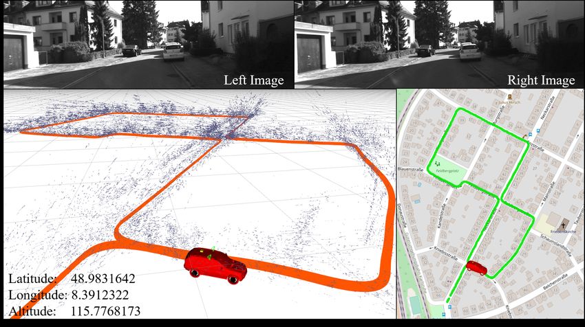
                                         into a global coordinate. Meanwhile, the accumulated drifts          Fig. 1.   KITTI dataset results of the proposed sensor fusion framework
                                         are eliminated. We evaluate the performance of our system            (VO + GPS). The top of this figure is a pair of stereo images. The left
                                         on public datasets and with real-world experiments. Results          bottom part is the estimated trajectory and feature points, while the right
                                         are compared against other state-of-the-art algorithms. We           bottom part is the estimated global trajectory aligned with Google map.
                                         highlight that our system is a general framework, which can
                                         easily fuse various global sensors in a unified pose graph
                                         optimization. Our implementations are open source1 .

                                                               I. I NTRODUCTION
                                                                                                              long run. Although some vision-based loop closure methods
                                            Autonomous robot has become a popular research topic
                                                                                                              were proposed to eliminate drifts, they cannot handle the
                                         over the last decades. We have seen an increasing demand for
                                                                                                              large-scale environment with the mass data.
                                         robots in various applications, such as autonomous driving,
                                         inspection, search and rescue. One of the fundamental tech-             Compared with local sensors, global sensors, such as
                                         nologies for autonomous tasks is localization. Robots require        GPS, barometers, and magnetometers, have advantages in
                                         precise 6-DoF (Degrees of Freedom) poses for navigation              global localization within large-scale environments. They
                                         and control. A lot of sesnors have been used for local pose          provide global measurements with respect to the fixed earth
                                         estimation. The Radar and LiDAR are widely used in the               frame, which is drift-free. However, their measurements
                                         confined indoor environment, while the camera and IMU are            are usually unsmooth and noisy, which cannot be directly
                                         applicable in both indoor and outdoor environments. There            used for precise control and navigation. Taking GPS as an
                                         are many impressive algorithms for local pose estimation,            example, it can measure approximate location in meters, but
                                         such as visual-based method [1]–[5], and visual-inertial-            measurements are discontinuous at a low rate. Also, it only
                                         based method [6]–[11]. These algorithms achieves incre-              measures 3D position without 3D orientation. Therefore,
                                         mental and accurate state estimation within a local region.          only global sensors are insufficient for real-time 6-DoF state
                                         However, there are several drawbacks limiting the usage of           estimation.
                                         these algorithms in practice.                                           Since local sensors (camera, IMU and LiDAR) achieves
                                            The first drawback of local pose estimation algorithems           impressive performance in local accuracy and global sensors
                                         is that they produce pose estimation in a local frame (with          (GPS, magnetometer and barometer) are drift-free, it is a
                                         respect to the starting point) without a global coordinate. We       smart way to fuse them together to achieve locally accurate
                                         may get different estimations when we start from different           and globally drift-free 6-DoF pose estimation. In order to
                                         points even in the same environment. Hence, they are un-             increase the robustness, we want to fuse sensors as many as
                                         friendly to reuse without a fixed global coordinate. The sec-        possible. Consequently, a general framework which supports
                                         ond drawback is that due to the lack of global measurements,         multiple sensors is required. Although traditional EKF-based
                                         the local estimations are prone to accumulated drifts in the         methods can fuse the local estimation into the global frame
                                                                                                              gradually, an accurate initial guess about the transformation
                                           All authors are with the Department of Electronic and              between different frames is required to guarantee conver-
                                         Computer Engineering, Hong Kong University of Science and            gence. Also, the EKF methods are sensitive to time synchro-
                                         Technology, Hong Kong, China. {tong.qin, shaozu.cao,
                                         jie.pan}@connect.ust.hk, eeshaojie@ust.hk.                           nization. Any late-coming measurements will cause trouble
                                           1 https://github.com/HKUST-Aerial-Robotics/VINS-Fusion             since states cannot be propagated back in filter procedure.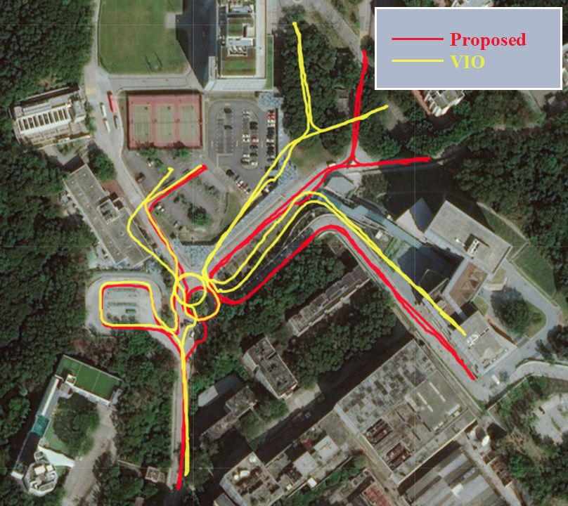
Fig. 2. An illustration of the proposed framework structure. The global estimator fuses local estimations with various global sensors to achieve locally
accurate and globally drift-free pose estimation.

To this end, we use an optimization-based method to solve                     Due to the lack of global measurement, the accumulated
this problem, which is suitable for multiple sensor fusion                    drifts is unavoidable over time.
inherently.                                                                      For global-aware localization, global sensors (GPS, mag-
   In this paper, we propose an optimization framework to                     netometer, barometer, etc) are incorporated in the system.
fuse local estimations with global sensor measurements. Lo-                   Global sensor measures absolute quantities with respect
cal estimations come from existing state-of-the-art VO/VIO                    to the earth frame, which are independent of the starting
works. Global sensors are treated as general factors in pose                  point. Global measurements are usually noisy and low-
graph. Local factors and global sensor factors are summed                     frequency, so they cannot be used alone. Therefore, global
up together to build the optimization problem. Our system                     sensors are usually fused with local sensors for accurate
achieves locally accurate and globally drift-free state estima-               and global-aware localization. [18] proposed an EKF-based
tion. We highlight the contribution of this paper as follows:                 algorithm to fuse visual measurement with inertial and GPS
   • a general framework to fuse various global sensors with                  measurement to get drift-free estimation. [19] used UKF
      local estimations, which achieves locally accurate and                  (Unscented Kalman Filter) algorithm to fuse visual, LiDAR
      globally drift-free localization.                                       and GPS measurements, which is an extension of EKF
   • an evaluation of the proposed system on both public                      without analytic Jacobians. Filter-based methods are sensitive
      datasets and real experiments.                                          to time synchronization. Any late-coming measurements
   • open-source code for the community.                                      will cause trouble since states cannot be propagated back
                                                                              in filter procedure. Hence, special ordering mechanism is
                       II. R ELATED W ORK                                     required to make sure that all measurements from multiple
   Recently, multiple sensor fusion approach for state esti-                  sensors are in order. Compared with filter-based method,
mation has become a popular trend in order to improve both                    optimization-based method have advantage in this aspect.
accuracy and robustness. By the type of sensors employed                      Because the big bundle serves as a nature buffer, it can
in the system, research works can be classified as local                      wait and store measurements for a long time. [20] used
localization and global-aware localization.                                   an optimization-based framework to fuse local VIO (Visual
   For local localization, cameras, IMU, LiDAR and RGB-D                      Inertial Odometry) with GPS measurements, which produced
sensors are usually used for 6-DoF state estimation in small                  more accurate results than method proposed in [18]. The
environment. Impressive approaches over the last decades                      transformation between local coordinate and global coordi-
include visual-based methods [1]–[5], LiDAR-based methods                     nate was frequently optimized in this approach. Few research
[12], RGB-D based methods [13], and event-based methods                       works fuse sensors more than three types. In this paper,
[14]. There are also some multi-sensor fusion methods, such                   we propose a more general optimization-based framework
as visual-inertial fusion [6]–[11, 15, 16] and visual-LiDAR                   for global localization, which can support multiple global
fusion [17]. Among these work, [6, 7, 9] are filter-based                     sensors. Each sensor serves as a general factor, which can
methods while [8, 10, 11] are optimization-based methods. In                  be easily added into the optimization problem.
optimization-based framework, a lot of visual measurements
and inertial measurements are kept in a bundle. The states                                         III. S YSTEM OVERVIEW
related to the observed measurements are optimized together.                     According to the measurement’s reference frame, we cat-
One advantage of optimization-based approaches over EKF-                      egory sensors into local and global types.
based ones is that states can be iteratively linearized to in-                   1) Local Sensors: Camera, LiDAR, IMU (accelerometer
crease accuracy. Both filter-based methods and optimization-                  and gyroscope), etc. This kind of sensor is not globally
based methods can achieve highly accurate state estimation.                   referenced, thus a reference frame is usually needed. In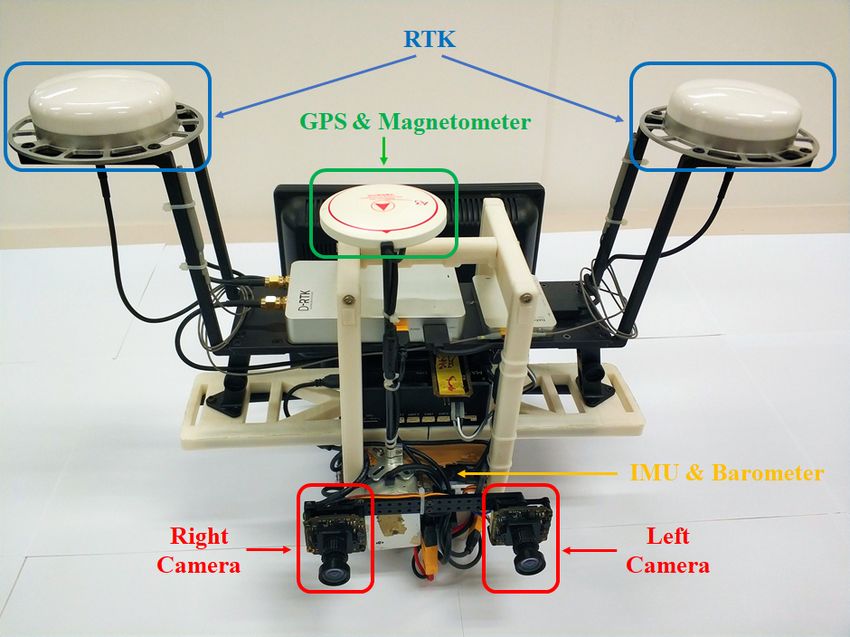
general, the first pose of the robot is set as the origin in order
to boot up the sensor. The estimation of the robot’s pose
incrementally evolves from the starting point. Therefore,
accumulated drift will grow with the distance from starting
point.
2) Global Sensors: GPS, magnetometer, barometer, etc.
This kind of sensor is globally referenced. It always works
under a fixed global frame, such as the earth frame. The Fig. 3. An illustration of the global pose graph structure. Every node
origin of the reference frame is fixed and known in advance. represents one pose in world frame, which contains position and orientation.
Their measurements are global-referenced but noisy. The The edge between two consecutive nodes is a local constraint, which is from
local estimation (VO/VIO). Other edges are global constraints, which come
error is independent of traveled distance. For GPS, it mea- from global sensors.
sures absolute longitude, latitude and altitude with respect
to the earth. The longitude, latitude, and altitude can be
converted to x, y and z coordinate. For magnetometer, it
c
measures magnetic field direction and strength, which can where rB (ẑbbk+1
k
, X ) and rC (ẑl j , X ) represent inertial and
determine the orientation. For barometer, it measures air visual residuals respectively. The prior term, {rp , Hp },
pressure, which can be converted to height. contains information about past marginalized states. ρ(·)
The structure of our framework is shown in Fig. 2. Local represents robust huber norm [21]. The detailed explanation
sensors (camera and IMU) are used in local estimation. The can be found at [11]. The VIO achieves accurate real-time
existing VO/VIO approaches are adopted to produce local 6-DoF pose estimations in the local frame.
poses. Local results and global sensors are input into a global B. Global Pose Graph Structure
pose graph. They are converted to unified factors to construct
The illustration of the global pose graph structure is shown
the optimization problem. The global estimator generates
in Fig. 3. Every pose, which contains position and orientation
locally accurate and globally aware 6-DoF pose results.
in world frame, serves as one node in the pose graph.
IV. M ETHODOLOGY The density of nodes is determined by the lowest-frequency
sensor. The edge between two consecutive nodes is a local
A. Local Pose Estimation
constraint, which is from local estimation (VO/VIO). That
For local pose estimation, we adopt existing VO (Vi- edge constrains the relative pose from one node to another
sual Odometry)/VIO (Visual-Inertial Odometry) algorithms. node. Other edges are global constraints, which come from
There are many impressive VO/VIO algorithms, such as global sensors.
[4, 6]–[11]. Any of them can be used as local pose estimation The nature of pose graph optimization is an MLE (Max-
in our framework, as long as it produces 6-DoF poses. This imum Likelihood Estimation) problem. The MLE consists
part is not the main contribution of this paper. For the com- of the joint probability distribution of robot poses over
pleteness, we briefly introduce our previous VIO algorithm a time period. Variables are global poses of all nodes,
[11], which is used in our open-source implementations. X = {x0 , x1 , ..., xn }, where xi = {pw w
i , qi }. p
w
and
The VIO estimates poses of several IMU frames and w
q are position and orientation under the global frame.
features’ depth within a sliding window. The states are Under the assumption that all measurement probabilities are
defined as: independent, the problem is typically derived as,
Xl = [x0 , x1 , · · · xn , λ0 , λ1 , · · · λm ] Yn Y
(1) X ∗ = arg max p(zkt |X ), (3)
xk = plbk , vbl k , qlbk , ba , bg , k ∈ [0, n],
X t=0 k∈S
where the k-th IMU state xk consists of the position plbk , where S is the set of measurements, which includes local
velocity vbl k , orientation qlbk of IMU’s center with respect to measurements (VO\VIO) and global measurments (GPS,
local reference frame l. We use quaternion to represent orien- magnetometer, barometer and so on). We assume the uncer-
tation. The first IMU pose is set as reference frame. ba and tainty of measurements are Gaussian distribution with mean
bg are accelerometer bias and gyroscope bias respectively. and covariance, which is p(zkt |X ) ∼ N (z̃kt , Ωkt ). Therefore,
Features are parameterized by their inverse depth λ when the above-mentioned equation is derived as,
first observed in camera frame. The estimation is formulated n Y
Y 1 2
as a nonlinear least-squares problem, X ∗ = arg max exp(− zkt − hkt (X ) Ωk )
X t=0 k∈S
2 t
( n X (4)
2
X
k k 2
= arg min zt − ht (X ) Ωk .
2
X
min krp − Hp X k + rB (ẑbbkk+1 , X ) b
+ X t
Xl Pbk t=0 k∈S
k∈B k+1
(2) 2
The Mahalanobis norm is krkΩ = rT Ω−1 r. Then the state
X c 2
ρ( rC (ẑl j , X) c )
Pl j
, estimation is converted to a nonlinear least squares problem,
(l,j)∈C which is also known as Bundle Adjustment (BA).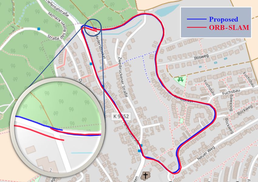
C. Sensor Factors                                                             of measurement differs zw a lot, we set a big covariance.
    1) Local Factor: Since the local estimation (VO/VIO) Otherwise, we use a small covariance.
is accurate within a small region, we take advantage of                          4) Barometer Factor: The barometer measures the air
the relative pose between two frames. Considering two                         pressure   in an area. We assume that the air pressure is
sequential frame t − 1 and frame t, the local factor is derived               constant  at  one altitude over a period of time. So the air
as,                                                                           pressure  can  be converted to height linearly. As the same as
                                                                              GPS, we set the first measurement as the origin height. Then
                                                                              we get the measurement of height ztm . Intuitively, the factor
zlt − hlt (X ) = zlt − hlt (xt−1 , xt )
                    l −1 l                  w −1 w                       is a residual of height estimation, which is written as:
                     qt−1 (pt − plt−1 )           qt−1 (pt − pw      t−1 )
                 =               −1
                           qlt−1 qlt                   qw
                                                             −1 w           ,           zm      m         m      m          m
                                                                                          t − ht (X ) = zt − ht (xt ) = zt − zt .        (8)
                                                         t−1 qt
                                                                       (5) Since this measurement is noisy, we caculate the variance of
                                                                              several measurments within a short time, and use it in the
where (qlt−1 , plt−1 ) and (qlt , plt ) are poses at time t − 1 and
                                                                              cost function.
t in local frame from VO/VIO.                 is the minus operation
                                                                                 5) Other Global Factors: Though we only specify GPS,
on the error state of quaternion. The first row represents
                                                                              magnetometer, and barometer factors in detail, our system is
relative position error between two poses, and the second
                                                                              not limited to these global sensors. Other global sensors and
row represents relative rotation error between two poses. If
                                                                              even some artificial sensors, such as Motion Capture system,
the VO/VIO algorithm produces the covariance matrix of
                                                                              WiFi and Bluetooth fingerprint, can be used in our system.
poses, we use it as the covariance of local measurements.
                                                                              The key is to model these measurements as residual factors
Otherwise, we use the unified covariance for all local mea-
                                                                              under one global frame.
surments.
    2) GPS Factor: Raw measurements of GPS are longitude, D. Pose Graph Optimization
latitude, and altitude, which are not in x,y, and z-axis
                                                                                 Once the graph is built, optimizing it equals to finding
coordinates. Generally, we can convert longitude, latitude
                                                                              the configuration of nodes that match all edges as much as
and altitude into ECEF (Earth Centred Earth Fixed), ENU
                                                                              possible. Ceres Solver [22] is used for solving this nonlinear
(local East North Up), and NED (local North East Down)
                                                                              problem, which utilizes Gaussian-Newton and Levenberg-
coordinates. Here, we take ENU coordinate as the example.
                                                                              Marquadt approaches in an iterative way.
By setting the first GPS measurement as the origin point, we
                                                                                 We run pose graph optimization at low frequency (1Hz).
get GPS’s measruments in the ENU world frame, pGP               t
                                                                     S
                                                                        =
                                                                              After  every optimization, we get the transformation for
[xw      w w T
    t , yt , zt ] . The GPS factor is derived as,                             local frame to global frame. Therefore, We can transform
  zGPt
         S
           −hGPt
                  S
                    (X ) = zGP t
                                  S
                                    −hGP
                                       t
                                           S
                                             (xt ) = pGP
                                                       t
                                                           S
                                                             −pw  t . (6)
                                                                              subsequent high-rate local poses (VO/VIO, 200Hz) by this
                                                                              transformation to achieve real-time high-rate global poses.
The GPS measurements directly constrain the position of Since the pose graph is quite sparse, the computation com-
every node. The covariance is determined by the number plexity increases linearly with the number of poses. We
of satellites when the measurement is received. The more can keep a huge window for pose graph optimization to
satellites it receives, the smaller covariance it is.                         get accurate and globally drift-free pose estimation. When
    3) Magnetometer Factor: The magnetometer can measure the computation complexity exceeds real-time capability, we
a vector of the magnetic field intensity. The direction of this throw old poses and measurements, and keep the window in
vector can help to determine orientation in the world frame. a limited size.
We assume the magnetometer is calibrated offline without
offset or bias. First of all, we lookup table to get the magnetic                              V. E XPERIMENTAL R ESULTS
intensity zw of the local region in the ENU coordinate. We                       We evaluate the proposed system with visual and inertial
assume that the magnetic intensity zw is constant within this sensors both on datasets and with real-world experiments.
area. Our measurement is denoted as zm          t . The orientation of        In the first experiment, we compare the proposed algorithm
zmt    should    match  z w
                             if  we put  the  sensor  coinciding with with another state-of-the-art algorithm on public datasets. We
the ENU coordinate. Inspired by this, the factor is derived then test our system with self-developed sensor suite in the
as:                                                                           real-world outdoor environment. The numerical analysis is
              zm − hm (X ) = zm − hm (xt )                                    generated to show the accuracy of our system in detail.
            t      t           t      t
                            zm
                             t         w −1 z
                                              w                 (7)    A. Datasets
                          = m    − qm
                                    b qt         ,
                           kzt k           kzw k
                                                                          We evaluate our proposed system using KITTI
where qm  b is the transformation from robot’s center to               Datasets [23]. The datasets are collected onboard a
the magnetometer’s center, which is known and calibrated               vehicle, which contains stereo images (Point Grey Flea
offline. Since the magnetic field is easily affected by the envi-      2, 1382x512 monochrome, 10 FPS) and GPS. Images are
ronment, we only use the normalized vector without length.             synchronized and rectified. The transformation between
The length is used to determine covariance. If the length              sensors is calibrated. Also, the ground truth states are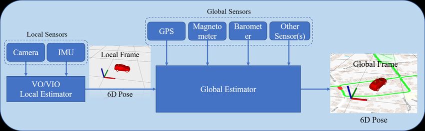
Relative Pose Error in 10_03_drive_0042
1.5
Translation Error [%] 1.4
Proposed
ORB-SLAM
1.3
1.2
1.1
200 300 400 500 600 700 800
Path Length [m]
0.015
Rotation Error [deg/m]
Proposed
0.01 ORB-SLAM
0.005
0
200 300 400 500 600 700 800
Path Length [m]
Fig. 6. Trajectories of one KITTI sequence (09 30 drive 0033) recovered
from ORB-SLAM and the proposed algorithm.
Fig. 4. Rotation error and translation error plot in 10 03 drive 0042.
TABLE I
Relative Pose Error in 09_30_drive_0033 RMSE [24] IN KITTI DATASETS IN METERS .
1
Translation Error [%]
Proposed
ORB-SLAM
0.8 RMSE[m]
Sequences Length[km]
ORB-SLAM Proposed
0.6
09 30 drive 0016 0.39 0.18 0.12
0.4 09 30 drive 0018 2.21 0.83 0.24
200 300 400 500 600 700 800 09 30 drive 0020 1.23 0.71 0.27
Path Length [m] 09 30 drive 0027 0.69 0.57 0.15
0.015 09 30 drive 0033 1.71 3.01 0.27
Rotation Error [deg/m]
Proposed 09 30 drive 0034 0.92 1.04 0.20
0.01 ORB-SLAM
10 03 drive 0027 3.72 1.25 0.28
10 03 drive 0042 2.45 12.48 0.63
0.005
0
200 300 400 500 600 700 800
Path Length [m]
Fig. 5. Rotation error and translation error plot in 09 30 drive 0033.
rotation angles, it cannot improve local accuracy on rotation.
The RMSE (Root Mean Square Errors) of absolute trajec-
tory error for more sequences in KITTI datasets is shown in
Table. I. Estimated trajectories are aligned with the ground
provided by the Inertial Navigation System (OXTS RT
truth by Horn’s method [25]. For all sequences, the proposed
3003). We run datasets with stereo cameras, latitude,
method outperforms orb-slam, which demonstrates that fus-
longitude, and altitude from raw GPS measurements. The
ing GPS measurements effectively increases the accuracy of
stereo cameras are used for local state estimation. The
the estimated trajectory. Intuitively, GPS corrects accumu-
local results are fused with GPS measurements in global
lated drifts in the long run.
optimization.
Trajectories of one KITTI sequence (09 30 drive 0033)
In this experiment, we compare our results with ORB-
recovered from ORB-SLAM and the proposed algorithm
SLAM [4], a state-of-the-art visual odometry method that
are shown in Fig. 6. Trajectories are aligned with Google
works with stereo cameras. Orb-slam is an optimization-
map from the bird-eye view. From the picture, we can see
based algorithm with powerful relocalization capability. It
that the estimated trajectory of ORB-SLAM drifts several
maintains a map of keyframes and landmarks. We evaluate
meters at the end. The estimated trajecotry of proposed
RPE (Relative Pose Errors) and ATE (Relative Trajecotry
method matches the road network well. This experiment
Error) one results produced by proposed method and ORB-
demonstrates that proposed system has advantage of pose
SLAM. The RPE is caculated by the tool proposed in [23].
estimation in a long distance.
The position and rotation RPE of two sequences are shown
in Fig. 4 and Fig. 5 respectively. For translation error, the
B. Real-world experiment
proposed method is obviously lower than ORB-SLAM. It
shows that the position drift is effectively eliminated by GPS In this experiment, we used self-developed sensor suite
measurement. For rotation error, the proposed method is not which were equipped with multiple sensors. The sensor suite
better than ORB-SLAM. Because GPS can’t directly measure is shown in Fig. 7. It contains stereo cameras (mvBlueFOX-Fig. 7. The sensor suite we used for the outdoor experiment,
which contains two forward-looking global shutter cameras (MatrixVision
mvBlueFOX-MLC200w) with 752x480 resolution. We use the built-in IMU, Fig. 10. The trajectories of our large-scale outdoor experiment recovered
magnetometer, barometer and GPS from the DJI A3 flight controller. from VIO and the proposed algorithm (VIO + GPS + magnetometer +
barometer) respectively.
Outdoor Trajecotry
20
VIO
MLC200w, 20Hz) and DJI A3 controller2 , which inculdes
15 Proposed
MSF
built-in IMU, magnetometer, barometer and GPS receiver.
10
RTK GPS We also equip it with RTK (Real-Time Kinematic)3 receiver
for high-accurate localization. The RTK base station is estab-
5
lished on the top of a building. The RTK can provide precise
positioning of one centimeter vertically and horizontally,
y [m]
0
which is treated as ground truth. We run states estimation
-5
with all available sensors.
-10 For accuracy comparison, we walked two circles on the
ground. We compare our results against MSF [18], which
-15
fuses visual odometry, inertial measurements, and GPS in an
-20
0 5 10 15 20 25 30
EKF-based framework. The trajecotry comparison is shown
x [m] in Fig. 8, and the RPE (Relative Pose Error) is plotted in
Fig. 9. We can see obvious translation drift in the estimated
Fig. 8. The trajectories of our small-scale outdoor experiment recovered trajectory of VIO. From the relative pose error, we can see
from VIO, the proposed algorithm and MSF respectively. We use RTK
trajectory as ground truth.
that the proposed system improved the accuracy of VIO a
lot. Also, the proposed system outperforms MSF [18]. The
RMSE of more outdoor experiments is shown in Table. II.
Relative Pose Error in Outdoor Dataset Our system achieved the best performance in all sequence.
1.5
VIO We also perform a larger outdoor experiment and com-
Translation error [m]
MSF
Proposed pared the results with Google map. Estimated trajecoties
1 are shown in Fig. 10. The estimated trajecotry of VIO
0.5
drifted along with distance. Thanks to the global sensors,
the trajectory of proposed system is almost drift-free, which
0
matches the road map very well.
2 10 30 60 80
Distance [m]
VI. C ONCLUSION
Fig. 9. Relative pose error plot in our small scale outdoor experiment. In this paper, we propose a optimization-based framework
to fuse local estimations with global sensors. Local estima-
TABLE II tions came from previous VO/VIO work. Global sensors are
RMSE[ M ] IN OUTDOOR EXPERIMENT. treated as general factors in pose graph optimization. This
system achieves locally accurate and globally drift-free pose
RMSE[m] estimation. We demonstrate the impressive performance of
Sequence Length[m]
VIO Proposed MSF our system on public datasets and with real-world experi-
Outdoor1 242.05 0.77 0.40 0.66 ments.
Outdoor2 233.89 0.66 0.41 0.58
Outdoor3 232.13 0.75 0.38 0.63 2 http://www.dji.com/a3
3 https://www.dji.com/d-rtkR EFERENCES [25] B. K. Horn, “Closed-form solution of absolute orientation using unit
quaternions,” JOSA A, vol. 4, no. 4, pp. 629–642, 1987.
[1] G. Klein and D. Murray, “Parallel tracking and mapping for small ar
workspaces,” in Mixed and Augmented Reality, 2007. IEEE and ACM
International Symposium on, 2007, pp. 225–234.
[2] C. Forster, M. Pizzoli, and D. Scaramuzza, “SVO: Fast semi-direct
monocular visual odometry,” in Proc. of the IEEE Int. Conf. on Robot.
and Autom., Hong Kong, China, May 2014.
[3] J. Engel, T. Schöps, and D. Cremers, “Lsd-slam: Large-scale di-
rect monocular slam,” in European Conference on Computer Vision.
Springer International Publishing, 2014, pp. 834–849.
[4] R. Mur-Artal, J. Montiel, and J. D. Tardos, “Orb-slam: a versatile and
accurate monocular slam system,” IEEE Trans. Robot., vol. 31, no. 5,
pp. 1147–1163, 2015.
[5] J. Engel, V. Koltun, and D. Cremers, “Direct sparse odometry,” IEEE
Transactions on Pattern Analysis and Machine Intelligence, 2017.
[6] A. I. Mourikis and S. I. Roumeliotis, “A multi-state constraint Kalman
filter for vision-aided inertial navigation,” in Proc. of the IEEE Int.
Conf. on Robot. and Autom., Roma, Italy, Apr. 2007, pp. 3565–3572.
[7] M. Li and A. Mourikis, “High-precision, consistent EKF-based visual-
inertial odometry,” Int. J. Robot. Research, vol. 32, no. 6, pp. 690–711,
May 2013.
[8] S. Leutenegger, S. Lynen, M. Bosse, R. Siegwart, and P. Furgale,
“Keyframe-based visual-inertial odometry using nonlinear optimiza-
tion,” Int. J. Robot. Research, vol. 34, no. 3, pp. 314–334, Mar. 2014.
[9] M. Bloesch, S. Omari, M. Hutter, and R. Siegwart, “Robust visual
inertial odometry using a direct ekf-based approach,” in Proc. of the
IEEE/RSJ Int. Conf. on Intell. Robots and Syst., 2015, pp. 298–304.
[10] R. Mur-Artal and J. D. Tardós, “Visual-inertial monocular slam with
map reuse,” IEEE Robotics and Automation Letters, vol. 2, no. 2, pp.
796–803, 2017.
[11] T. Qin, P. Li, and S. Shen, “Vins-mono: A robust and versatile
monocular visual-inertial state estimator,” IEEE Trans. Robot., vol. 34,
no. 4, pp. 1004–1020, 2018.
[12] J. Zhang and S. Singh, “Loam: Lidar odometry and mapping in real-
time.” in Robotics: Science and Systems, vol. 2, 2014, p. 9.
[13] C. Kerl, J. Sturm, and D. Cremers, “Dense visual slam for rgb-d
cameras,” in Proc. of the IEEE/RSJ Int. Conf. on Intell. Robots and
Syst.
[14] H. Rebecq, T. Horstschaefer, G. Gallego, and D. Scaramuzza, “Evo: A
geometric approach to event-based 6-dof parallel tracking and mapping
in real time,” IEEE Robotics and Automation Letters, vol. 2, no. 2,
pp. 593–600, 2017.
[15] G. P. Huang, A. I. Mourikis, and S. I. Roumeliotis, “Observability-
based rules for designing consistent ekf slam estimators,” Int. J. Robot.
Research, vol. 29, no. 5, pp. 502–528, 2010.
[16] H. Liu, M. Chen, G. Zhang, H. Bao, and Y. Bao, “Ice-ba: Incremental,
consistent and efficient bundle adjustment for visual-inertial slam,” in
Proc. of the IEEE Int. Conf. on Pattern Recognition, 2018, pp. 1974–
1982.
[17] J. Zhang and S. Singh, “Visual-lidar odometry and mapping: Low-
drift, robust, and fast,” in Proc. of the IEEE Int. Conf. on Robot. and
Autom. IEEE, 2015, pp. 2174–2181.
[18] S. Lynen, M. W. Achtelik, S. Weiss, M. Chli, and R. Siegwart,
“A robust and modular multi-sensor fusion approach applied to mav
navigation,” in Proc. of the IEEE/RSJ Int. Conf. on Intell. Robots and
Syst. IEEE, 2013, pp. 3923–3929.
[19] S. Shen, Y. Mulgaonkar, N. Michael, and V. Kumar, “Multi-sensor fu-
sion for robust autonomous flight in indoor and outdoor environments
with a rotorcraft MAV,” in Proc. of the IEEE Int. Conf. on Robot. and
Autom., Hong Kong, China, May 2014, pp. 4974–4981.
[20] R. Mascaro, L. Teixeira, T. Hinzmann, R. Siegwart, and M. Chli,
“Gomsf: Graph-optimization based multi-sensor fusion for robust
uav pose estimation,” in International Conference on Robotics and
Automation (ICRA 2018). IEEE, 2018.
[21] P. Huber, “Robust estimation of a location parameter,” Annals of
Mathematical Statistics, vol. 35, no. 2, pp. 73–101, 1964.
[22] S. Agarwal, K. Mierle, and Others, “Ceres solver,” http://ceres-solver.
org.
[23] A. Geiger, P. Lenz, and R. Urtasun, “Are we ready for autonomous
driving? the kitti vision benchmark suite,” in Proc. of the IEEE Int.
Conf. on Pattern Recognition, 2012, pp. 3354–3361.
[24] J. Sturm, N. Engelhard, F. Endres, W. Burgard, and D. Cremers, “A
benchmark for the evaluation of rgb-d slam systems,” in Proc. of the
IEEE/RSJ Int. Conf. on Intell. Robots and Syst., 2012, pp. 573–580.You can also read


