Using Unsupervised Learning for Data-Driven Procurement Demand Aggregation

PRELIMINARY PREPRINT VERSION: DO NOT CITE
 The AAAI Digital Library will contain the published
 version some time after the conference.

 Using Unsupervised Learning for
 Data-Driven Procurement Demand Aggregation
 Eran Shaham, 1 Adam Westerski, 2 Rajaraman Kanagasabai, 3 Amudha Narayanan, 4
 Samuel Ong, 5 Jiayu Wong, 6 Manjeet Singh7
 Institute for Infocomm Research, A*STAR, Singapore,1,2,3,4 ComfortDelGro, Singapore,5
 A*STAR Procurement Office, A*STAR, Singapore,6,7
 {eran-shaham, adam-westerski, kanagasa, naraa}@i2r.a-star.edu.sg,1,2,3,4 samuelong@comfortdelgro.com,5
 {wong_jiayu, manjeet_singh}@hq.a-star.edu.sg,6,7

 Abstract (Bartolini 2011). Knowing its magnitude, companies in-
 Procurement is an essential operation of every organization creasingly invest in optimizing procurement operations by
 regardless of its size or domain. As such, aggregating the de- reorganizing their practices to root out any inefficiencies or
 mands could lead to better value-for-money due to: (1) lower problems. This paper describes our experience in develop-
 bulk prices; (2) larger vendor tendering; (3) lower shipping ing an AI solution for demand aggregation and deploying it
 and handling fees; and (4) reduced legal and administration
 overheads. This paper describes our experience in developing in A*STAR, a large governmental research organization in
 an AI solution for demand aggregation and deploying it in Singapore with procurement expenditure in the scale of hun-
 A*STAR, a large governmental research organization in Sin- dreds of millions of dollars annually. We were presented
 gapore with procurement expenditure to the scale of hundreds with a set of digitalized procurement data and had to work
 of millions of dollars annually. We formulate the demand ag- with certain constraints, such as noisy, incomplete and un-
 gregation problem using a bipartite graph model depicting the
 relationship between procured items and target vendors, and labeled data scattered across multiple legacy data manage-
 show that identifying maximal edge bicliques within that ment systems. This is in contrast to academic literature
 graph would reveal potential demand aggregation patterns. which discusses different aspects of procurement manage-
 We propose an unsupervised learning methodology for effi- ment based on theoretical frameworks and strong assump-
 ciently mining such bicliques using a novel Monte Carlo sub- tions on data scale, labeling and consistency.
 space clustering approach. Based on this, a proof-of-concept
 prototype was developed and tested with the end users during Large enterprises like A*STAR spend millions on pur-
 2017, and later trialed and iteratively refined, before being chases of goods and services. Demand aggregation is the
 rolled out in 2019. The final performance achieved on past process of aggregating the demands for better value-for-
 cases benchmark was: 100% precision (all aggregation op- money due to: (1) lower bulk prices; (2) larger vendor ten-
 portunities identified by the engine were correct) and 71% dering; (3) lower shipping and handling fees; and (4) re-
 recall (the engine correctly identified 71% of the past aggre-
 gation exercises that were transformed into bulk tenders). duced legal and administration overheads.
 The performance for new opportunities pointed out by the en- Our key insight is in formulating the demand aggregation
 gine was 81% (i.e., 81% of the newly identified cases were problem using a bipartite graph model which depicts the re-
 deemed useful cases for potential bulk tender contracts in the lationship between procured items and target vendors. The
 future). Overall, the cost savings from the true positive con- need for an AI solution is mainly due to the dataset size.
 tracts spotted so far are estimated to be S$7 million annually.
 While small datasets could settle for eyeballing, datasets of
 moderate size are already hard to handle. In addition, em-
 Introduction ploying simple techniques (e.g., clustering) will not be ade-
 quate due to the “curse of dimensionality” (Bellman 1961;
Procurement is an essential operation of every organization Beyer et al. 1999; Kriegel, Kröger, and Zimek 2009). Thus,
regardless of its size, business domain, and sector (i.e., pri- for a solution to be successfully deployed on an unlabeled
vate or public). A typical procurement budget can be a sig- large dataset, and to successfully scale (the dataset might in-
nificant portion of total expenditure, up to 60% of revenues crease in size over time), unsupervised learning techniques

Copyright © 2021, Association for the Advancement of Artificial Intelli-
gence (www.aaai.org). All rights reserved.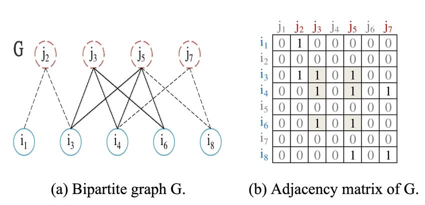

are required. We show that identifying maximal edge bi-
cliques within a bipartite graph would reveal potential de-
mand aggregation patterns. We propose an unsupervised
learning methodology for efficiently mining such bicliques
using a novel Monte Carlo subspace clustering approach.

We begin by describing the organizational context and the
problem description.

 Problem Description
A*STAR is a large governmental research organization in
Singapore comprising over 17 research entities and 5000
staff. Procurement spending of the organization can run into
hundreds of millions of dollars annually. Given their scale, Figure 1 Procurement workflow and steps.
the procurement operations are handled in a decentralized
manner by individual entities through an online workflow
 To fully appreciate the application, we first describe the pro-
comprising several steps (see Figure 1), and are governed
 curement data structure.
and audited by a centralized unit called the A*STAR Pro-
curement Office (A*PO) through a predominantly manual
process. Data Structure
 A*PO approached us in 2014 to create a data-driven The presented application was developed based on procure-
framework towards transforming the manual process of de- ment transactional data produced over the course of 8 years
tecting potential lapses, enhancing procurement compli- (from 2009 to 2016, inclusive). The dataset was refreshed in
ance, and optimizing procurement spend. We embarked on subsequent stages of the project to include consecutive
the A*STAR Procurement Analytics initiative to develop an years. However, to present a consistent and focused evalua-
AI platform for tackling three major challenges: (1) procure- tion scenario, including comparison of accuracy between
ment fraud detection; (2) procurement demand forecasting; different project stages, the experiments reported here relate
and (3) procurement demand aggregation. Our research on to the initial 8 years only.
the former two problems is reported elsewhere (Westerski Within this dataset, the key elements that comprise a pur-
et.al. 2015; Westerski, Kangasabai, and Sim 2017). chase are related to procedural stages of the procurement
 This paper focuses on the procurement demand aggrega- process as presented in Figure 1: (a) Invitation to Tender
tion problem and reports on our experience in developing an (ITT) or Invitation to Quotation (ITQ); (b) bid placement
AI solution for tackling the problem and deploying it and approval of selected supplier; and (c) issuance of Pur-
A*STAR-wide. Broadly, this was done in two phases: (1) a chase Order (PO). The data for typical final stages of pro-
proof-of-concept phase in 2017, where the core method was curement process related to delivery of goods and invoicing
developed by back testing on historical data; and (2) a pilot are generally treated as post-procurement process and are
trial and iterative refinement until final roll-out in 2019. A therefore not included in the discussion in this article. Also,
high-level description of the algorithm developed during the as demand aggregation applies only to orders that were suc-
proof-of-concept phase has been filed as a patent (Shaham, cessfully placed, we will focus on the PO data.
Westerski, and Kangasabai 2019). In this paper, we provide Each PO would point to an employee of the organization
a complete account of both the phases as part of sharing our fulfilling the role of buyer (requesting officer) and a hierar-
experiences. chy of approving officers (in charge of approving the pur-
 Demand aggregation is the process of aggregating the de- chase request). It would also have a creation date (day on
mands for goods and services to achieve better value-for- which requesting officer submitted the information to the
money in terms of: (1) lower bulk prices; (2) larger vendor system) and an approval date. A PO would further consist
tendering; (3) lower shipping and handling fees; and (4) re- of purchase order items, each of which can relate to a dif-
duced legal and administration overheads. Large enterprises ferent item or service and contain further details, such as:
such as A*STAR spend millions of dollars on purchases of textual item description, quantity of items bought and unit
goods and services. Thus, even a small change in these four price per single item. Similar structure of purchases split
fields could lead to substantial savings. into items with details of pricing, quantities, descriptions

etc. would also be present during earlier stages of (a) and
(b). It is worth noting that values at all stages can differ –
starting from expected purchases, to what suppliers offer, to
what was finally negotiated and approved.
 Throughout the experiments, we learned that the key fea-
tures that most influenced the capabilities of our algorithm
were the following five aspects of the procurement data:
who (requester); what (item description); what type (mate-
rial group); from who (vendor); and when (creation/ap-
proval date).
 In total, the dataset comprised 1,032,275 POs with
660,162 distinct items, and 14,834 unique vendors. On av-
erage, a single PO had 2.2 items attached. However, 59% of
the POs had only 1 order item attached, and 97% had 10 or
less. Within the remaining 3%, the maximal recorded
amount of order items per PO was 164. This reflects the
overall behavior of the organization employees and the pol-
icies in place, which focused on simple orders typically re-
lated to one type of good.
 Figure 2 Simplified example of a procurement database contain-
 ing hidden demand aggregation patterns (patterns can overlap).
 Application Description
Aggregating and analyzing the demand using the PO dataset
is not straightforward, due to the following challenges:
• Item description was a key field, but it was free text with
 no standard terminology. Also, it was of short length
 (

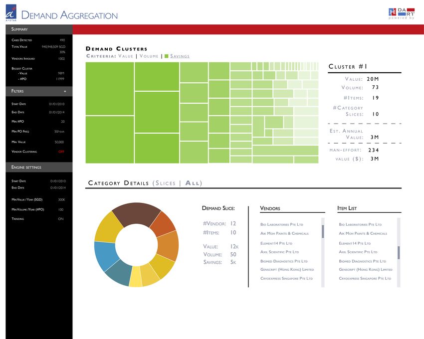
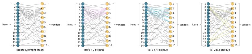
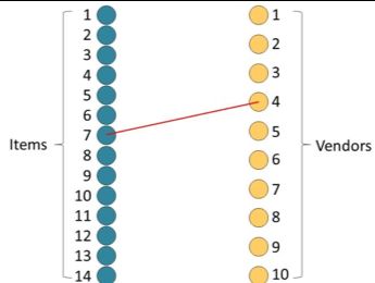
Figure 4 (a) Example of a procurement bipartite graph comprising: (b) biclique of 6 items x 2 vendors ({i2, i3, i4, i5, i6, i7} × {v2, v3});
 (c) biclique of 3 items x 4 vendors ({i2, i3, i4} × {v2, v3, v4, v5}); and (d) biclique of 2 items x 3 vendors ({i2, i13} × {v3, v6, v7}).

 was proved to be NP-complete (Garey and Johnson
 1979).
 3. µ(I, J) = |I| + |J| — known as the MAXIMUM VERTEX
 BICLIQUE problem. The problem can be solved in poly-
 nomial time using a minimum cut algorithm (Hochbaum
 1998; Garey and Johnson 1979).

 To achieve better value-for-money, demand aggregation
 aims to encapsulate the largest possible number of purchas-
 ing orders, and to “replace” them with one order. i.e., replace
 Figure 5 (a) Bipartite graph G; and (b) its corresponding adja- |I|×|J| individual purchasing orders (|I| items bought from |J|
cency matrix, comprising the maximum edge biclique ({i3, i4, i6}, vendors) with one purchasing order (which includes the |I|
 {j3, j5}) of size 6 edges and 5 vertices. items from e.g., the cheapest vendor). As such, in this paper
responding partition into two disjoint sets of vertices, a bi- we focus on the problem of finding the set of maximal edge
clique is a complete bipartite subgraph such that every ver- bicliques (potentially overlapping). Each such maximal
tex of the first partition is connected to every vertex of the edge biclique will serve as a potential demand aggregation.
second partition (see example in Figure 5, where a vertex set We propose an efficient Subspace Biclique Clustering for
{i3, i4, i6} and a vertex set {j3, j5} form a biclique). Mathe- Procurement (SBCP) algorithm to tackle this challenging
matically, the notion of biclique is defined as follows. problem. Extensive experimentations on artificial and real-
 world procurement datasets demonstrate the superiority of
Definition 1. Let G = (U ∪ V, E) be a bipartite graph, where our proposed SBCP algorithm over state-of-the-art tech-
U and V are two disjoint sets of vertices, and E is an edge niques.
set such that ∀(i,j) ∈ E, i ∈ U, j ∈ V. A biclique within G is
a couple (set pair) (I, J) such that I ⊆ U, J ⊆ V and ∀i ∈ I, j Use of AI Technology
∈ J, (i, j) ∈ E.
 We are now ready to present the SBCP algorithm. Firstly,
 The computational complexity of finding the maximum we describe a Monte Carlo algorithm for extracting a list of
biclique depends on the exact objective function used. In maximal bicliques. Next, we prove that the list contains op-
 timal bicliques. Finally, we present the run-time analysis of
contrast to the well-known maximum clique problem
 the algorithm.
(Makino and Uno 2004; Tomita, Tanaka, and Takahashi
2006), the maximum biclique problem has three distinct var-
 Finding Maximal Bicliques
iants, with the following objective function µ(I, J):
1. µ(I, J) = |I| × |J| — known as the MAXIMUM EDGE BI- For ease of readability, we adopt the graph’s adjacency ma-
 CLIQUE problem. The problem was proved to be NP- trix representation, defined as follows (see the example in
 complete (Lonardi, Szpankowski, and Yang 2006; Figure 5b, which is the adjacency matrix representation of
 Peeters 2003), and challenging to approximate (Ambühl, the bipartite graph G in Figure 5a).
 Mastrolilli, and Svensson 2011; Feige 2002; Feige and
 Kogan 2004; Goerdt and Lanka 2004; Peeters 2003). Definition 2. Let G = (U ∪ V, E) be a bipartite graph such
2. µ(I, J) = |I| , where |I| = |J| — known as the BALANCED that |U| = m, and |V| = n. The adjacency matrix X of graph
 COMPLETE BIPARTITE SUBGRAPH problem (also G is a [m × n] matrix such that Xi,j = 1 if (i,j) ∈ E and Xi,j =
 known as the balanced biclique problem). The problem 0 otherwise.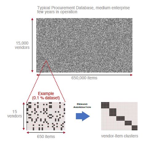

The input of the SBCP algorithm is therefore an adja-
cency matrix X of a given bipartite graph G, consisting of Algorithm 1: SBCP algorithm for extracting a list of
only boolean numbers, namely 0 and 1. The output of the maximal bicliques.
SBCP algorithm is a list of maximal bicliques, i.e., a list of
submatrices of ones, representing maximal bicliques within Input: X, a [m × n] matrix of boolean numbers.
G (the graph may contain multiple, possibly overlapping, Output: List of maximal bicliques.
maximal bicliques). The SBCP algorithm itself uses a sub- Initialization: Setting of N, |P| and |S| is discussed in
space clustering approach (Lonardi, Szpankowski, and the following section.
Yang 2006; Procopiuc et al. 2002; Shaham, Yu, and Li
2016). This common technique uses iterative random pro- 1: loop N times
jection (i.e., a Monte Carlo strategy) to obtain the biclique’s 2: // Seeding phase
seed, which is later expanded into a maximal biclique. 3: choose a subset of rows P uniformly at random;
 4: set I ← P, J ← ∅;
The SBCP Algorithm 5: // Interleaving row and column addition phase
 6: set isAddRow ← False;
Algorithm 1 presents the SBCP algorithm. As in the case of 7: set row i ← 1, column j ← 1;
many Monte Carlo algorithms, the structure of the SBCP al- 8: while row i ≤ m or column j ≤ n do
gorithm is very simple, and can be divided into the follow- 9: if isAddRow then // row addition
ing stages: 10: if Xi,J = 1 then
(i) Seeding (lines 2–4): a random selection of a set of rows 11: add i to I;
to serve as a seed of the maximal biclique. 12: i ← i + 1;
(ii) Addition of rows and columns (lines 5–20): interleaved 13: if j ≤ n then
accumulation of rows (lines 9–14) and columns (lines 15– 14: isAddRow ← !isAddRow
20), which comply with the rows and columns already accu- 15: else // column addition
mulated. 16: if XI,j = 1 then
(iii) Polynomial repetition (line 1): repetition of the above 17: add j to J;
two steps provides a probabilistic guarantee of acquiring a 18: j ← j + 1;
set of maximal bicliques. 19: if i ≤ m ⋀ (|J| ≥ |S| ⋁ j > n) then
 20: isAddRow ← !isAddRow
Remark 1. The Monte Carlo nature of the SBCP algorithm 21: return list of (I, J);
is revealed in phase (i) where random seeds are generated.
The subspace clustering nature of the SBCP algorithm is re-
vealed in phases (ii), where the seed of phase (i) is expanded
to form a maximal subset of rows over a maximal subset of Optimality of the Algorithm
columns, i.e., a maximal biclique. Clearly, the proposed SBCP algorithm can be viewed as a
 heuristic method. Next, we prove that there are solid theo-
Remark 2. To ease readability, lines 10 and 16 use the short retical reasons for this efficacy.
notations of: Xi,J = 1 and XI,j = 1, respectively, which have The SBCP algorithm derives inspiration from the BSC al-
the meaning of: ∀j ∈ J, Xi,j = 1 and ∀i ∈ I, Xi,j = 1, respec- gorithm (Shaham, Yu, and Li 2016). The motivation to en-
tively. hance the BSC algorithm is to avoid its tendency to be stuck
 in local maxima, which results in mining degenerated bi-
Remark 3. The SBCP algorithm has an inherent ability to cliques, i.e., bicliques that have large number rows but small
mine multiple, possibly overlapping, bicliques by utilizing number of columns (or the other way around, i.e., small
the independent random projection on each repetitive run, to number of rows and large number of columns). Such degen-
reveal columns and rows relevant only to a specific biclique. erated bicliques are less applicable, particularly in an indus-
 trial scenario usage such as demand aggregation. Next, we
Remark 4. The SBCP algorithm is not designed for the enu- outline the intuition behind the SBCP algorithm. For de-
meration of all maximal bicliques, which may be exponen- tailed argumentations, proofs, run-time analysis, and com-
tial in size (Eppstein 1994; Zhang et al. 2014). The algo- parisons to existing algorithms, we refer the reader to Sha-
rithm has a polynomial number of iterations, and thus, the ham, Yu, and Li (2016).
size of the return list is also polynomial. However, we next The intuition behind the BSC algorithm is that once we
prove that the returned list contains, with a fixed probability, successfully draw a discriminating column set (subset of the
optimal bicliques. rows), we can use it to collect the biclique’s columns, and
 only then, use the collected columns in order to collect the

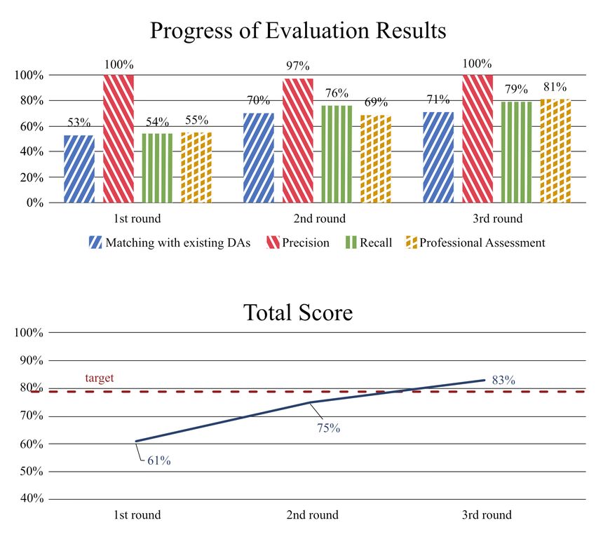
biclique’s rows. The mechanism behind the SBCP algorithm
is similar. Unlike the BSC algorithm which collects all of
the biclique’s columns and only then collects all of the bi-
clique’s rows, the SBCP algorithm collects the biclique’s
rows and columns in an alternating fashion. The intuition is
that an alternating expansion of the initial discriminating set
would result in an ever-growing discriminating set. This
promises better discriminating results (see Theorem 3.1 and
Experiment I (Shaham, Yu, and Li 2016)), which in turn
leads to a better detection probability (see Theorem 3.2
(Shaham, Yu, and Li 2016)), which results in an overall re-
duced run-time (see Subsection 3.3 (Shaham, Yu, and Li
2016)).

Run-time
The run-time is polynomial: mnO(1) (see Subsection 3.3
(Shaham, Yu, and Li 2016)).

 Application Use and Payoff Figure 6 Evaluation progress.

The implementation of the SBCP algorithm to create a prac- mined DAs from a past and future business perspective. The
tical procurement solution for A*PO was an iterative pro- evaluation of precision, recall and professional assessment
cess. Prior to achieving its final version, the solution under- employed an additional constraint: each was calculated
went three major rounds of evaluation. Each evaluation ran based on 30 randomly picked DAs out of all returned by the
the refined algorithm over a dataset of Purchasing Orders algorithm. Such methodology was necessary as the evalua-
(POs), passing the mined Demand Aggregation (DA) pat- tion of each pattern took considerable time and it was im-
terns, with their related POs, to a procurement officer for possible for A*PO staff to look through all detected patterns
evaluation. The quality of the algorithm was assessed using during each evaluation round.
the following metrics: (1) precision; (2) recall; (3) profes- For the first round of evaluation, we began with running
sional assessment of usefulness for newly detected and un- the SBCP algorithm on the entire A*STAR procurement da-
known DA patterns according to A*PO expertise; and (4) tabase for the years 2009 to 2016 (inclusive). To recall from
number of patterns matching with existing DAs, i.e., 33 pre- Section 2, the database comprises 660,162 items, 14,834
viously known DAs curated by A*PO legacy methods. For- vendors, and 1,032,275 POs.
mally, those are defined are follows: The evaluation by A*PO found various issues (e.g., price
 depreciation, coarse/grained clusters). Following A*PO
 feedback, we added domain constraints (encapsulating
1. =
 A*PO best practices) in the next two evaluation rounds:
 1. Use of only the most recent 3 years (i.e., years 2014–
2. = 2016). This resulted in a database comprising 271,219
 
 items, 7,319 vendors, and 391,671 POs.
 
3. = 2. Filter out patterns with less than 20 POs a year.
 
 3. Filter out patterns with a value less than S$70,000 a year.
 4. Filter out patterns with a descending price trend (trend
4. ℎ ℎ =
 calculated as linear regression).
 The above metrics were picked in order to reflect the rel- 5. Allow patterns to fail once on the above filters.
evant aspects of A*PO operations. Metrics (1) and (2) were
calculated with respect to POs within each detected pattern, After incorporating these new constraints, the SBCP
i.e., determining the quality of each pattern regardless to miner found 643 patterns. The final performance (see Figure
how many patterns were detected in total. Furthermore, the 6) achieved 71% detected legacy DAs (the existing DAs that
procurement officer would treat POs listed by the algorithm were not identified by the engine were A*PO manually
as a starting point, and further investigate using traditional crafted DAs, which violated A*PO-imposed domain con-
A*PO techniques whether other orders should have been in- straints). The performance for new DAs mined by the engine
cluded. Metrics (3) and (4) focus on the assessment of the was 81% (i.e., 81% of the newly identified DAs were

deemed by A*PO staff as useful cases for potential future
bulk tender contracts, to be thoroughly investigated by
A*PO). Furthermore, all POs assigned to the valid DAs
were correctly mined (100% precision); at the same time,
the valid DAs were determined 79% complete in terms of
listed POs in comparison to what the procurement officer
thought should have been reported (79% recall).
 A*PO calculated the estimation of the incurred savings
resulting from the usage of DAs, as follows. First, from a
chosen DA, a potentially discounted price is calculated as
the cheapest item price among an item subcluster. This is
repeated for all subclusters and subsequently for all DAs. In
the second step, the discounted price is computed by com-
paring with actual prices for items in the last 3 years. The
total savings were estimated to be > S$7 million, after ac-
counting for cost appreciation. Although this is an approxi-
mation, note that additional discounts from buying in bulk
and potential cost savings from reduced legal and admin-
istration overheads were not included. Thus, we believe the Figure 7 Dashboard analytics view.
estimate is quite conservative.
 Deployment Tweaks and Lessons Learned
Application Implementation and Deployment As part of our partnership, A*PO personnel were deeply in-
 volved in all stages of the project. Algorithmic decisions,
In practice, in a production scenario, new demand aggrega- such as to model the procurement dataset as a bipartite rela-
tion patterns need a rather lengthy time period in order to tionship graph and to use bicliques to represent demand ag-
surface. Therefore, at deployment stage the algorithm did gregation patterns, were explained to our collaborators.
not need to run constantly processing the stream of incom- Consequently, A*PO procurement officers were able to give
ing purchase orders in real-time. Instead, A*PO aimed to use us active feedback on refinements, which iteratively helped
the system as a decision-supporting mechanism for their an- to improve the algorithm’s performance. Although a number
nual management reports. At bootstrap, our system was used of these tweaks are hard to quantify, they were equally im-
to reveal past patterns from historical data which were un- portant for A*PO in terms of the deployment and practical
known to A*PO. Moving forward, as new purchases are use of the solution:
made and new data comes in, the system’s purpose is to give 1. Adjusting output to preference and analysis capability
suggestions of new/modified patterns to the procurement of- and capacity of the end users: during the first evaluation,
ficer; those patterns would subsequently be reviewed man- we discovered that our end users were overwhelmed by
ually by the officer and, if useful, recommend to manage- the amount of potential demand aggregation patterns. The
ment for new contracting/tendering decisions. To that end, SBCP algorithm, as other biclique mining algorithms,
the deployed application had the following characteristics as strives to deliver a complete set of all possible bicliques.
described below. However, in practical terms, this abundance turns out to
 be counterproductive to the end users, as it is too much to
Implementation digest. A constant communication of the results to the us-
 ers led to incorporating business rules, which helped to
The SBCP algorithm was implemented in Java 8, and de- trim and consolidate the demand aggregation patterns list,
ployed on a multi-core server running CentOS, using com- and to meet the end users’ needs and capacity.
mon libraries such as Apache 2.0 + LGPL, Commons Math, 2. The classic evaluation via precision and recall measure-
FastUtil and JavaCSV. ments did not turn out to be particularly relevant from a
 business standpoint of A*PO: the end users were not in-
Input/Output terested in patterns which in their understanding seemed
The input was extracted out of A*PO systems as a CSV for- obvious (i.e., patterns which could be established by a
 skilled procurement officer even without data examina-
mat comprising the following attributes: (1) requester name;
 tion or with little effort via BI tools). This resulted in a
(2) item description; (3) material group; (4) vendor name; ranking mechanism on top of the SBCP algorithm, which
and (5) creation/approval date. up-votes “interesting” and “non-obvious” patterns. The
 The output was also in the form of a CSV report format, criteria for those were discussed throughout the evalua-
accompanied by a dashboard analytics tool (see Figure 7). tions and involved incorporating additional data fields

(e.g., item categories, requesting officers, approving of- (Eppstein 1994), and bounding the biclique’s size (Liu et al.
 ficers, historical purchasing trends), in combination with 2006; Sanderson et al. 2003). Among the algorithms in the
 various thresholds and rules. last category we can find: reduction to maximal clique
3. Redefining requirements for the validity of DA patterns: (Makino and Uno 2004; Tomita, Tanaka, and Takahashi
 previous patterns curated manually by A*PO considered 2006), and reduction to frequent itemsets (Li et al. 2007;
 the aggregation of purchases across different material Uno, Kiyomi, and Arimura 2004; Zaki and Hsiao 2002).
 groups as valid. However, this turned out to be less valu- The reduction of the problem to finding a maximal clique
 able when using our algorithm, as it resulted in a greatly
 has the benefit of a well-researched field with an abundance
 increased number of patterns and generated patterns with
 weak business logic. Therefore, we enabled the output of heuristics and approximation algorithms (recall that the
 system to break down the mined DAs into their material problem is NP-complete (Peeters 2003)). However, in order
 groups’ components. to perform such reduction, an inflation of the bipartite graph
 is needed, which makes the problem computationally im-
 practical due to the large number of edges it adds.
 Maintenance The reduction of the problem to frequent itemsets bene-
 fits, as above, by relying on a rich field of research. How-
Future maintenance was an important criterion during the
 ever, it contains other difficulties. Literature has shown
application design. With a lean IT team supporting A*PO,
 (Zaki and Ogihara 1998) that a transactional database corre-
we designed the system with loosely coupled data applica-
 sponds to a bipartite graph G = (U ∪ V, E), where U is the
tion and UI layers, where the data exchange between the lay-
 set of items (itemsets), V is the set of transactions (tids), and
ers happens via CSV files in pre-defined formats. Thus, the
 E is the set of pairs (item, transaction), i.e., an edge in the
end users and supporting IT team have full flexibility in up-
 bipartite graph represents a transaction comprising the item.
dating the data feed into the application in view of future
 Take for example a set of products offered by a supermarket.
database upgrades and in maintaining the Tableau UI should
 A transaction would be a subset of products (itemset) pur-
there be new requirements.
 chased by a customer. Therefore, finding frequent itemsets
 Support for the application layer is currently provided by
 corresponds to finding bicliques, and finding a maximal fre-
our team. Our future plan is to license the technology to a
 quent closed itemset corresponds to finding a maximal bi-
local company to handle the technical support and mainte-
 clique. However, transforming a frequent itemset to a bi-
nance, and also productize it and commercialize further.
 clique, although requiring a trivial post-processing step, can
 be highly time consuming (Li et al. 2007). Therefore, these
 Related Work reductions to other domains may present practical and scala-
 bility problems (Zhang et al. 2014) and may not fully utilize
The MAXIMUM EDGE BICLIQUE problem has received the special characteristics of the bipartite graph.
much attention in academic research in recent years due to Out of other approximation work (Geerts, Goethals, and
its wide range of applications in areas such as bioinformatics Mielikäinen 2014), it is worth noting the problem of finding
(Ben-Dor et al. 2003; Cheng and Church 2000; Sanderson the number of edges to be deleted such that the resulting
et al. 2003), epidemiology (Mushlin et al. 2007), formal con- graph is a 2–approximation maximum edge biclique (Hoch-
cept analysis (Ganter and Wille 1999), manufacturing prob- baum 1998), and the finding of near complete bicliques (Li
lems (Dawande et al. 2001), molecular biology (Nussbaum et al. 2008; Liu, Li, and Wang 2008; Mishra, Ron, and
et al. 2010), machine learning (Mishra, Ron, and Swamina- Swaminathan 2003; Mishra, Ron, and Swaminathan 2004;
than 2003), management science (Swaminathan and Tayur Sim et al. 2006; Sim et al. 2009; Sim et al. 2011).
1998), database tiling (Geerts, Goethals, and Mielikäinen Zhang et al. (2014) introduced the iMBEA algorithm for
2004), and conjunctive clustering (Mishra, Ron, and the enumeration of maximal bicliques in a bipartite graph.
Swaminathan 2003). The algorithm uses an efficient branch-and-bound technique
 Most of the algorithms tackling the problem can be di- to prune away non-maximal subtrees of the search tree. De-
vided into the following three main categories: (i) exploita- spite the theoretical complexity of an exponential run-time,
tion of some class of graph; (ii) relaxation of the problem by the algorithm outperforms the previous state-of-the-art algo-
bounding a characteristic of a graph; and (iii) reduction to rithms: (i) MICA (Alexe et al. 2004) – the best known gen-
other domains. Among the algorithms in the first category eral graph algorithm; and (ii) LCM-MBC (Li et al. 2007) –
we can find: limitation to chordal bipartite graphs (Kloks a prime frequent closed itemsets algorithm (an improvement
and Kratsch 1995), and limitation to convex bipartite graphs of LCM (Uno, Kiyomi, and Arimura 2004) algorithm).
(Alexe et al. 2004; Kloks and Kratsch 1995; Nussbaum et Recent work by Shaham, Yu, and Li (2016) used a sub-
al. 2010). Among the algorithms in the second category we space clustering approach for finding the maximum edge bi-
can find: bounding the graph’s vertices degree (Alexe et al. clique in a bipartite graph. The algorithm, named BSC
2004; Liu et al. 2006), bounding the graph’s arboricity (Biclique Subspace Clustering), uses random projections to

obtain seed patterns, which are later grown into maximal so far are estimated to be S$7 million annually (this in addi-
edge bicliques. The repetitive projections ensure a probabil- tion to potential savings due to reduced legal and administra-
istic guarantee on the finding of the maximum edge biclique. tion overheads).
The algorithm is reported to be at least four orders of mag- As part of future work, we are exploring further improve-
nitude faster than the iMBEA algorithm on both artificial ments in accuracy and scalability of the core algorithm. In
and real-world datasets. addition, we plan to license the technology to a local com-
 To the best of our knowledge, only a few papers have pany to handle the technical support and maintenance, and
been published in the specific field of demand aggregation productize and commercialize it further.
for procurement (Chew 2017; Chowdhary et al. 2011; Wang
and Miller 2005). These papers use a naïve one-dimension
aggregation strategy, which suffers from the “curse of di- References
mensionality” (Bellman 1961; Beyer et al. 1999; Kriegel, Alexe, G.; Alexe, S.; Crama, Y.; Foldes. S.; Hammer, P. L.; and
Kröger, and Zimek 2009), and from sensitivity to text de- Simeone, B. 2004. Consensus Algorithms for the Generation of All
scriptions variability and the effectiveness of the similarity Maximal Bicliques. Discrete Applied Mathematics 145(1): 11–21.
measure used. Ambühl, C.; Mastrolilli, M.; and Svensson, O. 2011. Inapproxima-
 bility Results for Maximum Edge Biclique, Minimum Linear Ar-
 rangement, and Sparsest Cut. SIAM Journal on Computing 40(2):
 Conclusions and Future Work 567–596.
 Bartolini, A. 2011. Innovative Ideas for the Decade, Technical Re-
Aggregating procurement demands could lead to better port. Ardent Partners Research.
value-for-money and substantial cost savings for large or- Bellman, R. 1961. Adaptive Control Processes: A Guided Tour.
ganizations. This paper describes our experience in devel- Princeton, NJ: Princeton University Press.
oping an AI solution for demand aggregation and deploying Ben-Dor, A.; Chor, B.; Karp R.; and Yakhini, Z. 2003. Discovering
it in A*STAR, a large governmental research organization Local Structure in Gene Expression Data: The Order-Preserving
in Singapore with procurement expenditure in the scale of Submatrix Problem. Journal of Computational Biology 10 (3-4):
 373–384.
hundreds of millions of dollars annually.
 We formulate the demand aggregation problem using a Beyer, K.; Goldstein, J.; Ramakrishnan, R.; and Shaft, U. 1999.
 When is “Nearest Neighbor” Meaningful?. In Proceedings of the
bipartite graph model depicting the relationship between International Conference on Database Theory, 217–235. Berlin,
procured items and target vendors. We then show that iden- Heidelberg: Springer Berlin Heidelberg.
tifying maximal edge bicliques within that graph would re- Cheng Y., and Church G. M. 2000. Biclustering of Expression
veal potential demand aggregation patterns. We propose an Data. In Proceedings of the International Conference on Intelligent
unsupervised learning methodology for efficiently mining Systems for Molecular Biology, 93–103. Palo Alto, CA: AAAI
such bicliques using a novel Monte Carlo subspace cluster- Press.
ing approach. While the method can be viewed as an effec- Chew, T. H. 2017. Procurement Demand Aggregation. In Business
tive heuristic, we show that there is a strong theoretical base Analytics: Progress on Applications in Asia Pacific, edited by J. L.
 C. Sanz, 664–684. Singapore: World Scientific.
for its efficacy. The algorithm enhances the BSC algorithm.
 Chowdhary, P.; Ettl, M.; Dhurandhar, A.; Ghosh, S.; Maniachari,
As such, not only it inherits the theoretical analysis, but also G.; Graves, B.; Schaefer, B.; and Tang, Y. 2011. Managing Pro-
achieves lower complexity bounds and higher detection curement Spend Using Advanced Compliance Analytics. In Pro-
probability. ceedings of the IEEE International Conference on e-Business En-
 A proof of concept prototype was developed and tested gineering, 139–144.
with the end users during 2017, and later trialed and itera- Dawande, M.; Keskinocak, P.; Swaminathan, J. M.; and Tayur, S.
tively refined, before being rolled out in 2019. The final per- 2001. On Bipartite and Multipartite Clique Problems. Journal of
 Algorithms 41(2): 388–403.
formance achieved on past cases benchmark was: 71% of
past DAs transformed into bulk tenders were correctly de- Eppstein, D. 1994. Arboricity and Bipartite Subgraph Listing Al-
 gorithms. Information Processing Letters 51(4): 207–211.
tected by the engine. The performance for new opportunities
pointed out by the engine was 81% (i.e., 81% of the newly Feige, U. 2002. Relations Between Average Case Complexity and
 Approximation Complexity. In Proceedings of the ACM Sympo-
identified cases were deemed useful cases for potential bulk sium on Theory of Computing, 534–543. New York, NY: Associ-
tender contracts in the future). Additionally, per each valid ation for Computing Machinery.
DA identified, the engine achieved (in terms of POs) 100% Feige, U.; and Kogan, S. 2004. Hardness of Approximation of the
precision (all aggregated POs identified by the engine were Balanced Complete Bipartite Subgraph Problem, Technical Report
correct), and 79% recall (the engine correctly identified 79% MCS04-04. The Weizmann Institute of Science.
of POs that should have been put into the DAs). Overall, the Ganter B., and Wille, R. 1999. Formal Concept Analysis. Berlin,
direct cost savings from the true positive contracts spotted Heidelberg: Springer Berlin Heidelberg.
 Garey, M. R, and Johnson D. S. 1979. Computers and Intractabil-
 ity: A Guide to the Theory of NP-Completeness. W. H. Freeman.

Geerts, F.; Goethals, B.; and Mielikäinen, T. 2004. Tiling Data- Procopiuc, C. M.; Jones, M.; Agarwal, P. K.; and Murali, T. 2002.
bases. In Proceedings of the International Conference on Discov- A Monte Carlo Algorithm for Fast Projective Clustering. In Pro-
ery Science, 278–289. Berlin, Heidelberg: Springer Berlin Heidel- ceedings of the International Conference on Management of Data,
berg. 418–427.
Goerdt, A., and Lanka, A. 2004. An Approximation Hardness Re- Sanderson, M. J.; Driskell, A. C.; Ree, R. H.; Eulenstein, O.; and
sult for Bipartite Clique. Technical Report 48. Electronic Collo- Langley, S. 2003. Obtaining Maximal Concatenated Phylogenetic
quium on Computation Complexity. Data Sets from Large Sequence Databases. Molecular Biology and
Hochbaum, D. S. 1998, Approximating Clique and Biclique Prob- Evolution 20(7): 1036–1042.
lems. Journal of Algorithms 29(1): 174–200. Shaham, E.; Yu, H.; and Li, X. L. 2016. On Finding the Maximum
Kloks, T., and Kratsch, D. 1995. Computing a Perfect Edge With- Edge Biclique in a Bipartite Graph: A Subspace Clustering Ap-
out Vertex Elimination Ordering of a Chordal Bipartite Graph. In- proach. In Proceedings of the SIAM International Conference on
formation Processing Letters 55(1): 11–16. Data Mining, 315–323.
Kriegel, H. P.; Kröger, P. and Zimek, A. 2009. Clustering High- Shaham, E.; Westerski, A.; and Kangasabai, R. 2019. Method and
Dimensional Data: A Survey on Subspace Clustering, Pattern- Apparatus for Procurement Demand Aggregation. International
Based Clustering, and Correlation Clustering. ACM Transactions Patent No. WO2019231390A1.
on Knowledge Discovery from Data 3(1): 1–58. Sim, K.; Li, J.; Gopalkrishnan, V.; and Liu, G. 2006. Mining Max-
Kunegis, J. 2013. KONECT – The Koblenz Network Collection. imal Quasi-Bicliques to Co-Cluster Stocks and Financial Ratios for
In Proceedings of the International Conference on World Wide Value Investment. In Proceedings of the International Conference
Web Companion, 1343–1350. New York, NY: Association for on Data Mining, 1059–1063.
Computing Machinery Sim, K.; Li, J.; Gopalkrishnan, V.; and Liu, G. 2009. Mining Max-
Li, J.; Liu, G.; Li, H.; and Wong, L. 2007. Maximal Biclique Sub- imal Quasi-Bicliques: Novel Algorithm and Applications in the
graphs and Closed Pattern Pairs of the Adjacency Matrix: A One- Stock Market and Protein Networks. Statistical Analysis and Data
to-One Correspondence and Mining Algorithms. Transactions on Mining 2 (4): 255–273.
Knowledge and Data Engineering 19(12): 1625–1637. Sim, K.; Liu, G.; Gopalkrishnan, V.; and Li, J. 2011. A Case Study
Li, J.; Sim, K.; Liu, G.; and Wong, L. 2008. Maximal Quasi-Bi- on Financial Ratios via Cross-Graph Quasi-Bicliques. Information
cliques with Balanced Noise Tolerance: Concepts and Co-Cluster- Sciences 181(1): 201–216.
ing Applications. In Proceedings of the SIAM International Con- Swaminathan, J. M., and Tayur, S. R. 1998. Managing Broader
ference on Data Mining, 72–83. Product Lines Through Delayed Differentiation Using Vanilla
Liu, G.; Sim, K.; and Li, J. 2006. Efficient Mining of Large Maxi- Boxes. Management Science 44(12): 161–172.
mal Bicliques. In Proceedings of the International Conference on Tomita, E.; Tanaka, A.; and Takahashi, H. 2006. The Worst-Case
Data Warehousing and Knowledge Discovery, 437–448. Time Complexity for Generating All Maximal Cliques and Com-
Liu, X.; Li, J.; and Wang, L. 2008. Quasi-Bicliques: Complexity putational Experiments. Theoretical Computer Science 363(1):
and Binding Pairs. In Proceedings of the International Computing 28–42.
and Combinatorics Conference, 255–264. Uno, T.; Kiyomi, M.; and Arimura, H. 2004. LCM ver. 2: Efficient
Lonardi, S.; Szpankowski, W.; and Yang, Q. 2006. Finding Biclus- Mining Algorithms for Frequent/Closed/Maximal Itemsets. In Pro-
ters by Random Projections. Theoretical Computer Science ceedings of the ICDM Workshop on Frequent Itemset Mining Im-
368(3): 217–230. plementations 126.
Makino, K., and Uno, T. 2004. New Algorithms for Enumerating Wang, G. and Miller, S. 2005. Intelligent Aggregation of Purchase
All Maximal Cliques. In Proceedings of the Scandinavian Work- Orders in E-Procurement. In Proceedings of the IEEE International
shop on Algorithm Theory, 260–272. EDOC Enterprise Computing Conference, 27–36.
Melkman, A. A., and Shaham, E. 2004. Sleeved CoClustering. In Westerski, A.; Kangasabai, R.; Wong, J.; and Chang H. 2015. Pre-
Proceedings of the ACM SIGKDD International Conference on diction of Enterprise Purchases Using Markov Models in Procure-
Knowledge Discovery and Data Mining, 635–640. ment Analytics Applications. Procedia Computer Science 60:
 1357-1366.
Mishra, N.; Ron, D.; and Swaminathan, R. 2003. On Finding Large
Conjunctive Clusters. In Proceedings of the 16th Annual Confer- Westerski, A.; Kangasabai, R.; and Sim, K. 2017. Method of De-
ence on Learning Theory and 7th Kernel Workshop, 448–462. tecting Fraud in Procurement and System Thereof. International
 Patent No. WO2017116311A1.
Mishra, N.; Ron D.; and Swaminathan, R. 2004. A New Concep-
tual Clustering Framework. Machine Learning 56: 115–151. Zaki, M. J., and Hsiao, C. J. 2002. CHARM: An Efficient Algo-
 rithm for Closed Itemset Mining. In Proceedings of the Interna-
Mushlin, R. A.; Kershenbaum, A.; Gallagher, S. T.; and Rebbeck, tional Conference on Data Mining, 457–473.
T. R. 2007. A Graph-Theoretical Approach for Pattern Discovery
in Epidemiological Research. IBM Systems Journal 46(1): 135– Zaki M. J., and Ogihara, M. 1998. Theoretical Foundations of As-
149. sociation Rules. In Proceedings of the Workshop on Research Is-
 sues on Data Mining and Knowledge Discovery, 71–78.
Nussbaum, D.; Pu, S.; Sack, J. R.; Uno, T.; and Zarrabi-Zadeh, H.
2010. Finding Maximum Edge Bicliques in Convex Bipartite Zhang, Y.; Phillips, C. A.; Rogers, G. L.; Baker, E. J.; Chesler, E.
Graphs. In Proceedings of the International Computing and Com- J.; and Langston, M. A. 2014. On Finding Bicliques in Bipartite
binatorics Conference, 140–149. Graphs: A Novel Algorithm and its Application to the Integration
 of Diverse Biological Data Types. BMC Bioinformatics 15(1):
Peeters, R. 2003. The Maximum Edge Biclique Problem is NP- 110–127.
Complete. Discrete Applied Mathematics 131(3): 651–654.