Virtual Reality Simulations of Curved Spaces
←
→
Page content transcription
If your browser does not render page correctly, please read the page content below
Virtual Reality Simulations of Curved Spaces
arXiv:2011.00510v1 [physics.ed-ph] 1 Nov 2020

                                                                              Jeff Weeks

                                                                          November 3, 2020

                                                                               Abstract
                                                 Previous virtual-reality simulations of curved space, which typically
                                                 present honeycombs or other periodic structures, have proven effective
                                                 in letting mathematicians experience curved space directly. By con-
                                                 trast, for students and other non-mathematicians, a game like Non-
                                                 Euclidean Billiards is more effective because it gives students not just
                                                 something to see, but also something to do in the curved space. How-
                                                 ever, such simulations encounter a geometrical problem: they must
                                                 track the player’s hands as well as her head, and in curved space the
                                                 effects of holonomy would quickly lead to violations of body coherence.
                                                 This is, what the player sees with her eyes would disagree with what
                                                 she feels with her hands. The present article presents a solution to the
                                                 body coherence problem, as well as several other questions that arise
                                                 in interactive VR simulations in curved space.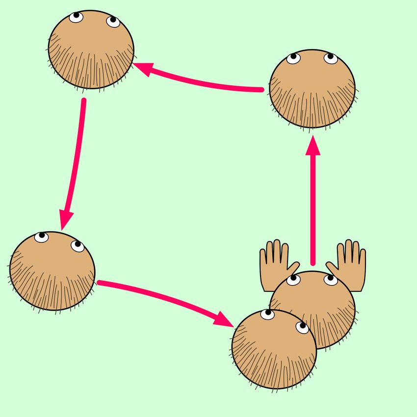
1 Introduction
Seeing curved spaces on a computer monitor is informative and fun, but
being in a curved space is a far richer experience and far more informative.
Indeed, for me personally, even having studied curved spaces for 45 years,
when I first put on the virtual reality (VR) headset and “visited” the 3-sphere
and hyperbolic 3-space, I found surprises. And after playing a few games of
billiards in those spaces (Figure 1), I got an intuitive feel for them unlike any
I had ever had before. The reason for that deeper gut-level understanding is
that VR connects not only with our conscious minds, but it also completely
hijacks our subconscious understanding of our environment: it feels real!
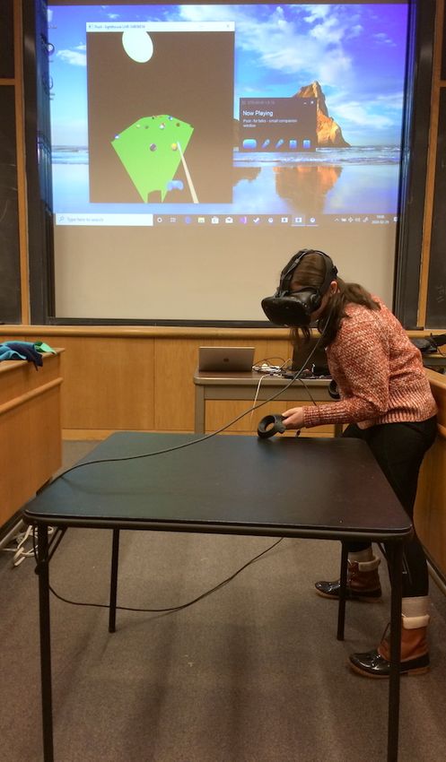
Figure 1: In hyperbolic 3-space, the billiards table is a regular pentagon
with all 90◦ angles (right). The table agrees locally with a square Euclidean
table in the lab (left), which adds a tactile component to the simulation for
greater realism.
2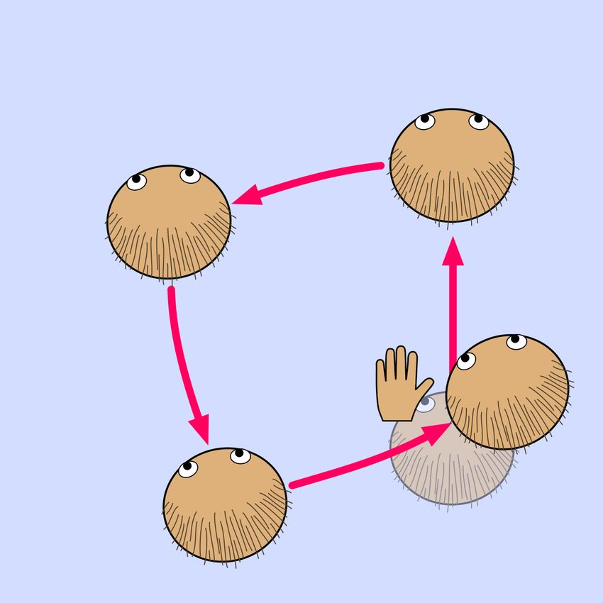
1.1   Why billiards?
Non-Euclidean Billiards offers two advantages over earlier curved-space VR
simulations:

   • Familiarity. Until now, curved-space VR simulations have presented
     abstract mathematical structures such as honeycombs. Such structures
     are fine for mathematicians, who use the structure’s periodicity to help
     understand the nature of the space. But when non-mathematicians
     see an unfamiliar structure in an unfamiliar space, the novelty of the
     structure often hides the novelty of the space. The present project
     instead presents familiar objects—a billiards table, billiard balls, a cue
     stick, and a lamp—so that the familiarity of the objects may illuminate,
     not hide, the novel properties of the space.

   • Interactivity. Previous curved-space VR simulations have been largely
     passive, which is fine for mathematicians who are already motivated
     to have a look around and think about what they’re seeing. Non-
     mathematicians, however, come to understand the properties of curved
     space more easily and more deeply when they’re given not only some-
     thing to see, but also something to do. In the Non-Euclidean Billiards
     app, the player is invited to put on the VR headset and play billiards
     for as long as she wants. The unhurried nature of a billiards game gives
     the player plenty of time to reflect on what she sees. Most importantly,
     the need to line up a good shot forces the player to continually walk
     around the table and look at the ball positions and the table itself from
     many different viewpoints.

The author and one of his colleagues are currently making plans for an en-
richment unit for 7th –12th grade students that will build on the familiarity
and interactivity of Non-Euclidean Billiards to teach some fundamental con-
cepts of curved space—namely angle sums, geodesic convergence/divergence,
curvature (defined as angle deficit per unit area), and holonomy—in a more
structured way.

                                      3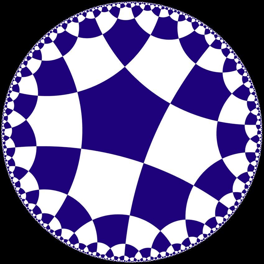
1.2   Structure of this article
I have chosen to present the mathematics of Non-Euclidean Billiards in a
pair of companion articles. The two articles share a common theme, but are
written for very different audiences. The first article [Weeks 2020] appears
in the proceedings of the conference
                          Bridges Aalto 2020
        Mathematics, Art, Music, Architecture, Education, Culture
Given the unusual breadth of that audience, I wrote that first article to
present the basic concepts of curved space, along with its surprising optical
effects, in the most visual and least technical way possible. All implementa-
tion details were omitted.
    By contrast, the present article is an account of my lecture at the Septem-
ber 2019 workshop
                     Illustrating Geometry and Topology
whose participants were my fellow illustrators of geometry. They, like the
readers of Experimental Mathematics, were already well acquainted with the
geometry of curved space, so I took the opportunity to dive “under the hood”
and explain recent progress in making curved-space VR simulations more in-
teractive, pedagogically effective, and internally efficient. The present article
provides a written account of this progress, for the benefit of other math-
ematicians who write curved-space VR simulations, both now and in the
future. The most substantive—and most surprising—discovery is the need
for a visitor to curved space to use her muscles to provide internal resistance
to the effects of holonomy, in order to maintain body coherence.
    Sections 2 and 3 explain body coherence in detail, and propose a strategy
for dealing with it in a VR simulation. Section 4 reviews the sequence of
mappings used in curved-space graphics, and offers some small conceptual
improvements that make working with them easier. Section 5 explains how
stereoscopic vision would lead a Euclidean-born tourist to grossly misjudge
distances in curved space. That same section then goes on to recommend
that curved-space VR apps be written to simulate distances as each space’s
native-born inhabitants perceive them, and shows how to modify the se-
quence of mappings from section 4 to achieve that goal. Finally, section 6
reviews the state of the art in simulating spaces that are homogeneous but
anisotropic.
    This project as a whole takes its inspiration from, and builds upon, the
pioneering work of [Hart et al. 2017a].

                                       4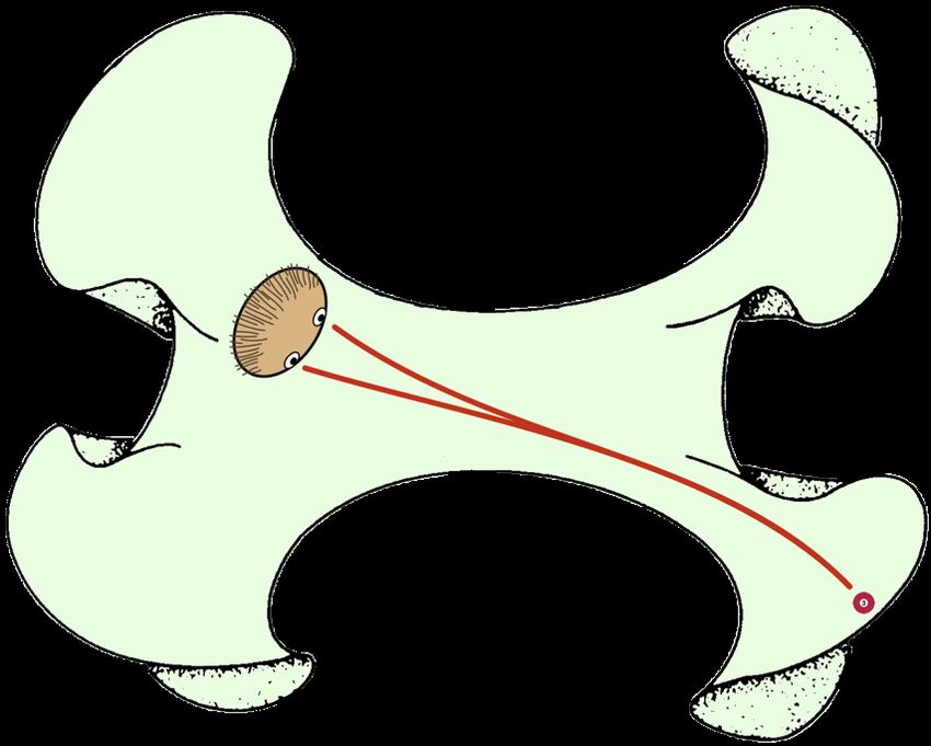
2    Headset tracking and body coherence: the prob-
     lem
When simulating a curved space in VR, a fundamental question is how to
map a pose of the user’s headset in the physical lab to a pose of the user’s
virtual self in the curved space. The simplest algorithm would be to map
local motions of the headset (as measured in its own local coordinate system)
to the same local motions of the user’s virtual head (as measured in its own
local coordinate system). In other words, if the physical headset moves 1 cm
to the left in the lab, the user’s virtual head moves 1 cm to the left in the
curved virtual space; if physical headset rotates 2◦ , the user’s virtual head
rotates 2◦ ; and so on.
    That naive algorithm would work fine if we were tracking only the user’s
head. But in practice we must track the user’s two hands as well, so that,
for example, a player in the Non-Euclidean Billiards game can take a shot.
Unfortunately holonomy can force the player’s head and hands out of align-
ment when using the naive tracking algorithm. To see how, consider what
happens if the player parallel-translates her head a small distance d forward,
then the same distance to her left, the same distance backwards, and finally
the same distance to right. In the physical Euclidean lab, her head returns
to its original position and orientation (Figure 2). But in the 3-sphere, those
forward, leftward, backward, and rightward motions are realized not by Eu-
clidean translations, but by rotations of the 3-sphere. If we place the player
at the north pole (0, 0, 0, 1) and let θ = d/R, where R is the radius of the

Figure 2: The player moves her head around a small square in the physical
Euclidean lab, while leaving her body and hands still.

                                      5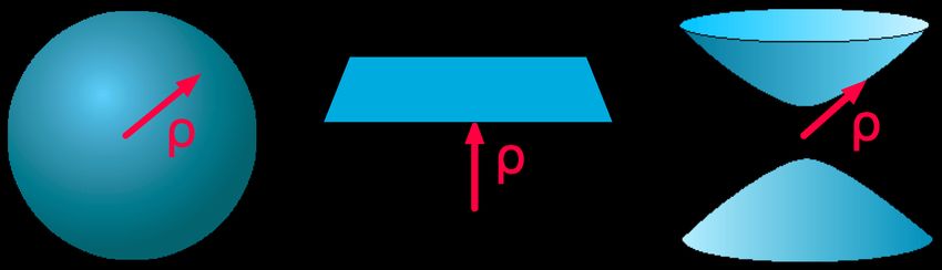
3-sphere, the final placement of the player’s head is given by the matrix
product
cos θ 0 0 − sin θ 1 0 0 0 cos θ 0 0 sin θ 1 0 0 0
0 1 0 0 0
cos θ 0 sin θ
0 1 0 0 0
cos θ 0 − sin θ
0 0 1 0 0 0 1 0 0 0 1 0 0 0 1 0
sin θ 0 0 cos θ 0 − sin θ 0 cos θ − sin θ 0 0 cos θ 0 sin θ 0 cos θ
This product assumes the left-to-right convention in which matrices act as
(row vector)(first factor)(second factor). . .
but may also be sensibly interpreted using the right-to-left convention
. . . (second factor)(first factor)(column vector)
Either way, the matrices for the forward, leftward, backward, and rightward
motions of the player’s head get applied in the opposite order from which the
player makes those motions, which is somewhat counterintuitive but never-
theless correct. The distance d is typically small relative to the 3-sphere’s
radius R, in which case the matrix product multiplies out to approximately
3
1 θ2 0 − θ2
−θ2 1 0 − θ3
2
0 0 1 0
θ3 θ3
2 2 0 1
The entries in the bottom row tell us that the player’s virtual head ends
up offset from its original position by about 21 θ3 radians in both the x and
y directions, while the upper-left 3 × 3 block tells us that the player’s head
ends up rotated by an angle of approximately θ2 radians. While the absolute
offset is only a third-order effect, the offset as a fraction of the square’s width
θ, namely 21 θ3 /θ = 12 θ2 is a second-order effect, just like the rotation.
The preceding computation proves that when the player moves her head
around a small square in the physical Euclidean lab, as shown in Figure 2,
the naive head-tracking algorithm would move her virtual head around a
path in the 3-sphere like the one shown in Figure 3(a). In the hyperbolic
case, an analogous matrix product
cosh θ 0 0 sinh θ 1 0 0 0 cosh θ 0 0 − sinh θ 1 0 0 0
0 1 0 0 0
cosh θ 0 − sinh θ
0 1 0 0 0
cosh θ 0 sinh θ
0 0 1 0 0 0 1 0 0 0 1 0 0 0 1 0
sinh θ 0 0 cosh θ 0 − sinh θ 0 cosh θ − sinh θ 0 0 cosh θ 0 sinh θ 0 cosh θ
shows that the naive head-tracking algorithm would move the player’s virtual
head around a path in hyperbolic 3-space like the one shown in Figure 3(b).
6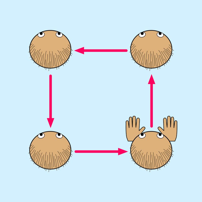
(a) Positive   holonomy   in   a       (b) Negative holonomy in hyper-
    3-sphere                               bolic 3-space

Figure 3: In a curved space, the player’s virtual head ends up offset and
rotated, by an amount proportional to the area that her path enclosed.

In both cases, when the player’s virtual head returns to the starting point
in the physical Euclidean lab, her virtual head ends up slightly offset and
slightly rotated relative to its original pose in the virtual curved space. In
and of itself that’s not a problem, but if she keeps her hands still while
moving her head, then she does have a problem: she sees her own hands
sitting slightly offset and slightly rotated (Figure 3), even though she still
feels her hands sitting straight in front of her (Figure 2).
    This discrepancy between what the player sees and what she feels, we call
body incoherence. It’s a challenging problem that all interactive curved-space
VR simulations, present and future, will face. Section 3 presents a solution
that works well in the case of Non-Euclidean Billiards, along with some more
general suggestions for other apps.

3    Headset tracking and body coherence: a solution
If you could truly visit hyperbolic 3-space or a 3-sphere, would you really
experience body incoherence? No, of course not. What you’d see and what
you’d feel would remain perfectly coherent. But as you parallel-translated
your head around in a small circle, you’d feel a slight torque in your neck.
You’d need to use your neck muscles to counter that torque, to keep your

                                       7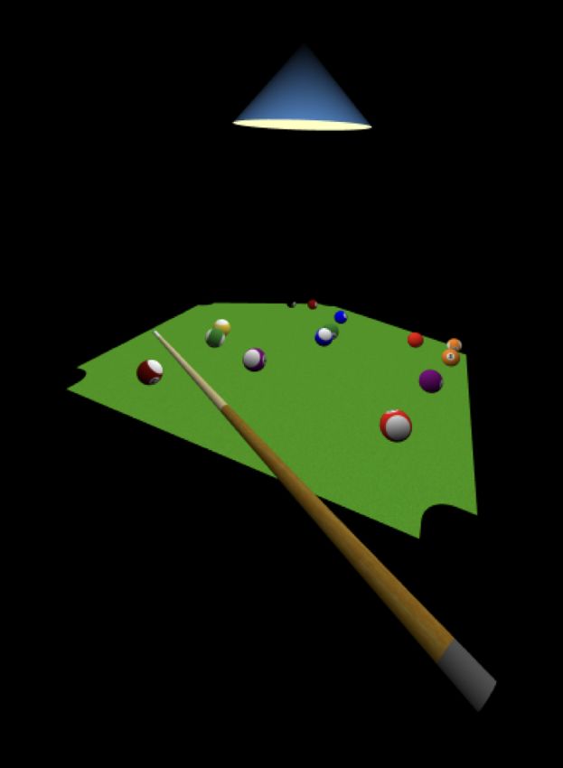
head pointed straight relative to your body. This mysterious uninvited
torque would feel roughly analogous to what you feel when you rotate a
spinning gyroscope about one axis and must apply a mysterious uninvited
torque to prevent the gyroscope from rotating about a perpendicular axis.
    Curved-space simulations, such as the Non-Euclidean Billiards game,
must pretend that the user’s neck is providing whatever torque is neces-
sary to keep her head aligned with her body. Hence we must abandon the
naive tracking algorithm and devise a new algorithm that’s guaranteed to
place the user’s head and hands coherently in the curved virtual space.

3.1   Tracking algorithm for Non-Euclidean Billiards
The Non-Euclidean Billiards game makes use of a square physical table (Fig-
ure 1(left)), which locally agrees with the virtual pentagonal (in H3 ) or trian-
gular (in S3 ) billiards table in the game (Figure 1(right)), and adds a tactile
component to the simulation. But the presence of this square physical table
means that we must also ensure coherence between where the player sees
the virtual table with her eyes and where she feels the physical table with
her hands. The simplest algorithm is to track each object—the player’s head
and each of her two hands—relative to the nearest edge of the physical table.
Although the algorithm applies equally well to each of the player’s hands,
the following paragraphs will describe it only for her head, for brevity.
    The algorithm expresses the player’s pose in the Euclidean lab relative to
a coordinate system attached to a nearby point on the edge of the physical
table, then transfers that pose to the simulated space by mapping into the
tangent space at the corresponding point on the corresponding edge of the
simulated table, and thence into the curved space itself via the exponential
map. This ensures that the simulated table edge that the player sees with
her eyes always agrees with the physical table edge that she feels with her
hands.
    At what point on the table edge should we base the aforementioned
tangent space? One might be tempted to use the closest point on the closest
edge, but this would introduce a small discontinuity: if the player stands
near a corner and leans forward with her head over the table itself, then as
she moves her head side to side, the “nearest edge point” may jump suddenly
from one edge of the table to the next, without passing through the corner
point. This jump in the basepoint for the tangent space would cause a
small—but potentially perceptible—jump in the headset’s position in the
simulated space. To avoid the discontinuous jump, one may instead base
the tangent space not at the nearest point on the nearest table edge, but

                                       8
rather at the table edge point whose azimuth agrees with the azimuth of the
player’s head, as seen from the center of the table.
    The preceding paragraphs define the mapping from the Euclidean physi-
cal space to the curved virtual space almost uniquely. The only free param-
eter is deciding which edge of the physical table corresponds to which edge
of the virtual table. The correspondence between the edges of the square
physical table and the edges of the virtual triangular, square or pentagonal
table is not fixed, but is something that must be traced around in real time,
as the player walks around the table. For example, if a player keeps walk-
ing around the physical table—always in the same direction, never turning
back—she’ll see the following edges in the following order:

        square physical table:     0 1 2 3 0 1 2 3 0 1 2 3 0 1 2 ...
        pentagonal virtual table : 0 1 2 3 4 0 1 2 3 4 0 1 2 3 4 . . .

This matching of an edge of the physical table to an edge of the virtual table
is the only thing that depends on the player’s history. Once that match-
ing is known, the headset’s pose in the Euclidean physical space uniquely
determines its pose in the curved virtual space, with no additional history
dependence.
    The same algorithm may be used to place each of the player’s hands in
the curved virtual space. This guarantees the coherence of the player’s body,
as well as its consistent placement relative to the table.

3.2   General principles
Looking to the future, all designers of interactive curved-space VR simula-
tions will face the body coherence problem. While a particular app’s ideal
solution may depend heavily on its context, some general principles apply:

   • Ensure visual stability. In a scene with no fixed reference points, it’s
     better to let the player’s virtual head move freely and tweak the player’s
     virtual hands to stay consistent with it, rather than to let the hands
     move freely and tweak the head to stay consistent. The reason for this
     is that artificially tweaking the player’s head would slightly shift her
     view of the whole scene. Hand motion alone must never affect how the
     player sees the scene, not even by the slightest amount. But if head
     motion causes a slight change in the position of the player’s hands,
     that would be undesirable but ultimately acceptable. This asymmetry
     is due to the primacy of the human visual system: a person’s sense
     of “where she is in the world” is tied most strongly to what she sees;

                                      9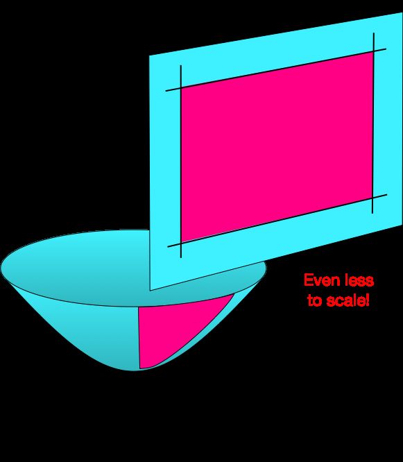
her hands and feet are then perceived as being 50–150 cm below that
      primary viewpoint.

    • Keep the player away from the walls. If the player in the Non-Euclidean
      Billiards game weren’t anchored to the table, then if she parallel-
      translated herself around a small circle several times, she’d see the
      virtual table orbit around her, eventually passing behind her back. At
      that point, if she turned around to face the table and take a shot, she’d
      risk walking into a wall of the physical lab (or, more likely, she’d see
      the “chaperone” bounds that the VR system inserts into the scene to
      prevent players from walking into walls). To avoid such a scenario, all
      curved-space VR apps should, if possible, keep their primary virtual
      content centered in middle of the physical lab, and keep the player’s
      position coherent with that primary content.

The most challenging curved-space VR apps to design may be those whose
game content is inherently large-scale, such as a potential VR version of
HyperRogue [Kopczyński et al. 2019]. Even games whose content may be
only a few meters across, such as the author’s 3D mazes in any of several
closed 3-manifolds, nevertheless appear infinite to the player, because the
player sees such a maze as an infinite periodic structure in the “universal
cover”, beckoning her to wander beyond the bounds of the fundamental do-
main (http://www.geometrygames.org/TorusGames). How might we let the
player travel longer distances than her real-world room would permit? One
solution would be to give her the ability to press a button and fly through
the scene, but that approach risks motion sickness, due to the player’s eyes
seeing accelerations that her inner ear doesn’t feel. A safer solution—one
used in some flat-space VR apps—would be teleportation: after selecting a
destination and pressing a button, the player “fades out” from her current
location, briefly sees total darkness, and then “fades back in” at her selected
destination.

4    Computer graphics in curved space
Most 3D graphics, whether in flat space or curved space, whether traditional
or VR (but excluding ray tracing and ray marching), relies on the following

                                      10
sequence of mappings:
Model Space −→ World Space
model
matrix
−→ Camera Space
view
matrix
−→ Projection Space
projection
transf ormation
Each object in the simulated world begins in its own local model space. The
model matrix places the object into a shared world space, along with all the
other objects. Conceptually one then places a camera into that same world
space, to take a picture of the various objects; in practice, though, one takes
the whole world and places it in front of the camera, in the camera’s own
camera space. Of course the camera—like a real physical camera—sees not
the whole space, but only the portion of it lying within a pyramid extending
from the camera’s lens outward. That pyramid gets further limited by a near
clipping plane and (optionally) a far clipping plane, leaving only objects
within the resulting view frustum visible. The projection transformation
maps the view frustum to a rectangular box in Euclidean 3-space.
An elementary exposition of computer graphics in S3 , E3 and H3 appears
in [Weeks 2002]. The following subsections summarize the essentials of that
article, but with a new approach to radians in the Euclidean case, a comment
on units in VR, a new way to visualize the projection transformation, and
an algorithm for drawing the “back hemisphere” in the spherical case.
4.1 Radians in S3 , E3 and H3
In the spherical case, the model, world, and camera spaces are all 3-spheres of
some desired radius ρ (Figure 4(left)). The 3-sphere is defined as a subset of
Euclidean 4-space E4 , where its radius is measured using the Euclidean metric
|(x, y, z, w)|2 = x2 + y 2 + z 2 + w2 = ρ2 .
The model and view matrices are elements of the orthogonal group O(4).
In the hyperbolic case, the model, world, and camera spaces are all hyper-
bolic 3-spaces of some desired radius ρ (Figure 4(right)). Hyperbolic 3-space
is defined as a subset of Minkowski space E3,1 , where its radius is measured
using the Minkowski metric
|(x, y, z, w)|2 = x2 + y 2 + z 2 − w2 = −ρ2 .
The model and view matrices are elements of the Lorentz group O(3, 1).
11Figure 4: The concept of radius applies not only to spheres (left), but also
to hyperbolic spaces (right) and even Euclidean spaces (center).
Surprisingly, it’s the Euclidean case that requires the greatest care. A
standard computer graphics trick is to take the coordinates (x, y, z) and
append a “1” as a fourth coordinate, so we can package up a rotation R and
a translation (∆x ∆y ∆z) as a single 4 × 4 matrix
R00 R01 R02 0
R10 R11 R12 0
(x y z 1)
R20 R21 R22 0
∆x ∆y ∆z 1
When you do the matrix multiplication, the “1” multiplies the ∆x ∆y ∆z and
they get added in. The awkward question here is: What are the units on ∆x,
∆y, and ∆z? If we’re measuring x, y, and z in meters, are ∆x, ∆y, and ∆z
also in meters? Yet the rotational components Rij are dimensionless. Few
mathematicians are comfortable having a transformation matrix with some
dimensionless entries and other entries in meters. The situation becomes
much clearer if instead of representing Euclidean 3-space as a hyperplane at
height w = 1, we represent it as a hyperplane at height w = ρ, and call ρ the
“radius” of this Euclidean space (Figure 4(center)). So now we can rewrite
our matrix product as
R00 R01 R02 0
R10 R11 R12 0
(x y z ρ)
R20
R21 R22 0
∆x/ρ ∆y/ρ ∆z/ρ 1
and it’s abundantly clear that ρ is in meters, just like x, y, and z, and ∆x/ρ,
∆y/ρ, and ∆z/ρ are dimensionless, just like the Rij . The best way to think
of this is that ∆x/ρ, ∆y/ρ, and ∆z/ρ are translation distances in Euclidean
radians.
12The big practical advantage to using Euclidean radians is that, by having
a purely dimensionless transformation matrix acting on a position vector
(x, y, z, ρ) in pure meters, we make the Euclidean case consistent with the
spherical and hyperbolic cases. So a game like Non-Euclidean Billiards can
often use exactly the same computer code for all three geometries, with no
need to split into separate cases.
4.2 VR needs explicit units
When writing traditional non-VR animations, most mathematicians (includ-
ing the author) treated distances as dimensionless quantities, in effect mea-
suring all distances in spherical, hyperbolic, or Euclidean radians. And that
was fine: in a non-VR maze in a 3-torus or a non-VR flight through a
Poincaré dodecahedral space, explicit units aren’t needed.
In VR, by contrast, units are essential. The player’s two eyes and two
hands are immersed in the simulated world, so the distances the player sees
with her eyes must agree with the distances she feels with her hands. The
player perceives herself as part of the scene, not as an onlooker peering into
a simulated world from the outside.
For an acceptable VR simulation, we must know (1) the space’s radius
of curvature in meters and (2) the size of each object in meters. To see why,
consider what happens when a player in a hyperbolic billiards game changes
the radius of curvature of the space. If she increases the radius of curvature,
the space as a whole will scale up, and any geometrical structures whose
size is tied to the radius of curvature will also scale up. For example, the
billiards table, which we’ve defined to be a right-angled regular pentagon,
will get larger. But the player’s body, whose size in meters is fixed, will
not get larger. Nor will the billiard balls, whose diameter is fixed at 57 mm,
nor the cue stick, whose length is fixed at 1 m. The final result is that when
the player increases the space’s radius of curvature, she’ll find herself playing
billiards on a larger right-angled pentagon, but with the same familiar billiard
balls and cue stick.
4.3 Visualizing the projection transformation
As part of the standard graphics pipeline, a vertex shader —sometimes more
correctly called a vertex function—computes and reports each vertex’s posi-
tion in homogeneous coordinates (x, y, z, w). The Graphics Processing Unit
(GPU) then divides through by the w-coordinate
x y z
(x, y, z, w) 7→ , , ,1
w w w
13to map the desired view frustum onto a rectangular box in the w = 1 hyper-
plane.
Even though the GPU really does divide through by w, and that’s how
computer graphicists think about it, I personally find it easier to think in
terms of dividing through by z instead. Dividing through by z makes the
geometrical meaning clearer. Moreover, essentially all vertex shaders apply a
90◦ rotation in the zw-plane, which sends our conceptually clear division-by-z
to the GPU’s hardwired division-by-w. Combining this with our convention
of letting ρ be the radius of the space even in the Euclidean case (Section 4.1),
the projection formula for all three geometries becomes
x y ρ
(x, y, z, ρ) 7→ , , 1,
z z z
In the Euclidean case, the division-by-z takes the view frustum to a
rectangular box, as desired (Figure 5). It’s perfectly acceptable to push
the frustum’s far wall off to infinity, thus mapping an infinite portion of a
pyramid onto a finite rectangular box. By constrast, if the frustum’s near
wall gets too close to the observer, it will push the rectangular box’s top face
upwards towards infinity, which quickly degrades the numerical precision of
the results as the floating-point arithmetic’s finite precision gets spread out
over an ever taller box.
Figure 5: In Euclidean graphics, dividing by z maps the view frustum to a
rectangular box (y coordinate suppressed).
14In the spherical case, that same division-by-z takes not a frustum, but
rather a solid I like to call the view banana (Figure 6), to a rectangular box.
Like a real banana, the view banana has flat sides and tapers down at both
ends.
In the hyperbolic case (Figure 7), we again map a frustum-like solid onto
a rectangular box, and again it’s perfectly acceptable to push the frustum’s
far wall off to infinity.
Figure 6: In spherical graphics, dividing by z maps the view banana to a
rectangular box (y coordinate suppressed).
Figure 7: In hyperbolic graphics, dividing by z maps the view frustum to a
rectangular box (y coordinate suppressed).
154.4 The 3-sphere
Rendering images in the 3-sphere is a two-part process. To see why, first
recall that in Euclidean graphics, if we let the near clipping distance go to
zero, the short edge of the red trapezoid in Figure 5 would approach the
observer (the black dot), which would send the top edge of its projected
image (the top edge of the red rectangle in the vertical plane) upwards to
infinity. To avoid that problem, in Euclidean graphics we always set the near
clipping distance to some ε > 0.
In spherical graphics, we face that same problem at both the top and
the bottom of the red view banana on the sphere in Figure 6. To avoid
trouble, we must set the near clipping distance to some ε > 0 to keep the
top edge of its projected image (the top edge of the red rectangle in the
vertical plane) from going upwards to infinity, and we must also set the far
clipping distance to π − ε to keep the bottom edge of the projected image
from going downwards to infinity.
One immediate consequence of this approach is that an ε-neighborhood
of the observer’s antipodal point is always excluded from the rendered image.
This is not surprising, given that a tiny fleck of dust sitting at the antipodal
point would fill the observer’s entire sky! While ray-tracing methods would
have no problem rendering the antipodal point, our mesh-based methods
always omit the antipodal point and some tiny neighborhood surrounding
it.
Our mesh-based methods can, however, easily see through the antipodal
point and render content that sits on the “back side” of the 3-sphere. That is,
we may render content whose line-of-sight distance from the observer falls in
the range [π + ε, 2π − ε]. Because the observer’s lines-of-sight all reconverge
at the antipodal point, what the observer sees at distances [π + ε, 2π − ε]
is precisely the same as what her antipodal twin would see at distances
[ε, π − ε]. In other words, to render the back hemisphere, we may simply
apply our usual methods to render what the antipodal twin sees at distances
[ε, π − ε]. Technical detail: the most efficient way to implement this on a
Tile-Based Deferred Render is to encode commands taking the 3-sphere’s
back hemisphere into the back half of the clipping box ( 12 ≤ z ≤ 1) and the
front hemisphere into the front half of the clipping box (0 ≤ z ≤ 12 ), and
then let the renderer process of the whole scene at once. That way back-
hemisphere objects that are eclipsed by front-hemisphere objects will never
get rendered at all.
If the observer’s head were perfectly transparent, would we also have to
render objects that she sees at distances in the range [2π+ε, 3π−ε]? No, this
16isn’t necessary, because these would be the same objects that the observer
sees at distances [ε, π − ε], and they would fill exactly the same portions of
observer’s sky.
5 Native-inhabitant view vs. tourist view
To focus on a distant object in hyperbolic 3-space, an observer must look
slightly cross-eyed, to compensate for the space’s inherent geodesic diver-
gence (Figure 8). For native inhabitants of hyperbolic space, this is fine,
because when they were babies they learned that a certain positive vergence
angle means that the object they’re looking at is far away. But a Euclidean-
born tourist who visits hyperbolic space would misinterpret that positive
vergence angle as meaning that the object is close. In fact the tourist would
see all of hyperbolic space crammed into a small ball, of radius only a meter
or two in the case of the hyperbolic Billiards game.
Figure 8: In hyperbolic space, an observer must look slightly cross-eyed to
focus on a distant object.
17Figure 9: In a 3-sphere, an observer must look “walleyed” to focus on objects
more than 90◦ away.
In a 3-sphere, by contrast, an observer must look less cross-eyed than in
Euclidean space, to compensate for the space’s inherent geodesic convergence
(Figure 9). When an object is exactly 90◦ away, like blue (#2) billiard ball
in Figure 9, the observer doesn’t need to look crosseyed at all. For those
of us who grew up in Euclidean space, our binocular vision makes that blue
(#2) ball seem infinitely far away. If a ball is more than 90◦ away, like the
red (#3) ball in Figure 9, the observer must look slightly “walleyed”—with
a negative vergence angle—to focus on it.
When designing a virtual reality simulation like the non-Euclidean bil-
lards game, the developer must decide whether to show the space the way
the native sees it, to show it the way the Euclidean-born tourist sees it, or
to offer the user the choice. For me, the tourist’s view is just too weird:
as you walk around hyperbolic 3-space, the entire contents of the universe
seem to move along with you, all trapped inside that finite ball. Spherical
space is even worse, because you have to look walleyed to focus on distant
objects. The human visual system can do this to some extent, but I person-
ally find it uncomfortable and vaguely distressing. To avoid such discomfort,
Non-Euclidean Billiards offers the native-inhabitant view only.
18To simulate a rigorously correct native-inhabitant view, we must trick
the user’s eyes and brain into perceiving each object’s true hyperbolic or
spherical distance. This is most easily accomplished by inserting an extra
step into the graphics pipeline:
Model Space −→ World Space
model
matrix
−→ Camera Space
view
matrix
−→ Euclidean Tangent Space
azimutal
equidistant
map
−→ Projection Space
projection
transf ormation
The extra step maps the simulation’s contents from the hyperbolic or spher-
ical camera space onto the observer’s Euclidean tangent space in such a
way that all distances from the observer’s head are preserved. In cartogra-
phy this is called an azimuthal equidistant map. In differential geometry it
could be called a logarithmic map because it’s the inverse of the exponential
map, but given the more common meanings of logarithmic and exponential,
those names feel awkward here. Note that the azimuthal equidistant map
gets computed relative to the observer’s head (more precisely, relative to the
bridge of her nose), not relative to each eye separately.
Unlike the preceding steps in the above pipeline, the azimuthal equidis-
tant map cannot be realized as a matrix multiplication. Fortunately, though,
it can be realized with a simple trigonometric computation, which puts only
a small extra burden on the vertex shader. For example, in the spherical
case, say an observer at P = (0, 0, 0, ρ) is viewing some point of interest
Q = (x, y, z, w) on a 3-sphere of radius ρ meters. Let θ be the distance in
radians from P to Q, and let d be that same distance in meters (measured
along the 3-sphere itself, not in the 4-dimensional ball that it bounds). We
want to find a point Q0 in the tangent space that sits in the same direction
from P as Q does, and also sits d meters away (but in the tangent space,
not on the 3-sphere). Geometrically it’s easy to see that
0 θ θ θ
Q = x, y, z, ρ .
sin θ sin θ sin θ
To compute θ, note that w = ρ cos θ, where w and ρ are both already known,
19so our shader code becomes
CosineTheta = clamp(w/rho, -1, +1)
Theta = acos(CosineTheta)
SineTheta = sin(Theta)
if SineTheta > 0.0001
Factor = Theta / SinTheta
else
Factor = 1 // correct near north pole,
// but not near south pole
Qprime = (Factor * x, Factor * y, Factor * z, rho)
The shader code for the hyperbolic case is essentially the same, but with
acosh and sinh instead of acos and sin, and different clamping bounds.
The above algorithm lets the observer use her Euclidean binocular vision
to see every point in the space at its correct hyperbolic or spherical distance.
This eliminates the illusion that all of hyperbolic space sits in a small finite
ball, and also eliminates the need for the observer to look walleyed in spher-
ical space. However, even though the observer perceives all objects at their
true hyperbolic or spherical distances, there’s still the rich and interesting
question of how the observer’s brain integrates those distances into a mental
model of the space. For a full discussion, see [Weeks 2020].
Note #1: In the spherical case, when rendering the back hemisphere we
must set Factor = (π + θ)/ sin θ in the shader code above, so that back-
hemisphere objects get drawn in the azimuthal equidistant map at distances
in the desired range [π + ε, 2π − ε].
Note #2: One of the referees has pointed out that the Hypernom VR game
[Hart et al. 2015] uses a technique similar to the one described here, but with
stereographic projection instead of the azimuthal equidistant map. Stereo-
graphic projection works well in Hypernom, which is a game for experiencing
the 3-sphere as a double-cover of the rotation group SO(3), rather than a
simulation of the 3-sphere for its own sake. However, because it grossly
distorts radial distances, stereographic projection would work poorly in a
game like Non-Euclidean Billiards, which strives to let players experience
the 3-sphere and hyperbolic 3-space as closely as possible to the way that
those spaces’ native inhabitants might experience them.
206 Thurston’s eight geometries
Thurston’s revolutionary Geometrization Theorem says that every closed
3-manifold may be cut into pieces in a natural way, and each piece will ad-
mit one of eight homogeneous geometries. Of the eight, the three isotropic
geometries S3 , E3 and H3 are the easiest to simulate. The product geometries
S2 × E, E2 × E (= E3 ) and H2 × E aren’t too much harder, with simulations
having been made first in traditional graphics [Weeks 2006] and more re-
cently in VR [Hart et al. 2017b]. Adding some “vertical shear” to each
product space gives a twisted product: twisted S2 × E (grouped with S3 in
the Geometrization Theorem, but with an extra free parameter to set the
amount of twist, which typically makes the geometry anisotropic), twisted
E2 × E (commonly known as Nil geometry) and twisted H2 × E (commonly
known as SL(2,
f R) geometry). The eighth geometry is called Sol geometry,
and is the strangest of all. Explicit geodesic computations have recently
been applied with great success to simulate the twisted product geometries
and even Sol [Berger 2015, 2017; Kopczyński et al. 2019, 2020; Novello et
al. 2020a, 2020b; Coulon et al. 2020a, 2020b, 2020c].
One could easily port the Non-Euclidean Billiards game to the prod-
uct geometries, and in fact I have already written a prototype of such
an app (Figure 10). However, I recommend against using the product
Figure 10: A pentagonal billiards table in H2×E. Even though its five edges
are perfectly straight, the player sees them as curved because of H2 × E’s
surprising optics. The more distant billiard balls appear slightly prolate for
the same reason.
21Figure 11: Straight lines don’t look straight.
geometries with general audiences, for the simple reason that straight lines
don’t look straight. The billiards game’s raison d’être is to introduce non-
mathematicians to curved space. In the case of hyperbolic geometry, the tra-
ditional approach to this task was to show people a picture of the Poincaré
disk model (Figure 11) and say that
the circular arcs are really straight lines in hyperbolic geometry,
but I’ve found this approach to be ineffective because non-mathematicians
think you’re saying that they should
pretend that the circular arcs are straight lines
(even though obviously they’re not).
When a hyperbolic billiard table is embedded in H2 × E, the table’s edges
and the balls’ trajectories, while intrinsically straight, nevertheless appear
curved to the player (Figure 10), because of the surprising optics of H2 × E
itself. This would make it very difficult to convince people that those edges
and trajectories really are straight, and that curved space is just as valid as
flat space. That’s why I wrote the Non-Euclidean Billiards game in H3 in-
stead, so players can see and feel the straightness of hyperbolic lines directly
(Figure 1). The same reasoning applies to favor S3 over S2 × E with general
audiences.
By contrast, with an audience of geometers and topologists, simulations
of all eight geometries are well received and provide much insight and food
for thought.
22Acknowledgements
I thank Sabetta Matsumoto for her generous and patient help getting me
started with virtual reality, and I thank the referees for their thoughtful
suggestions that greatly improved this article.
References
[Berger 2015] P. Berger. Espaces imaginaires, motifs et mirages. http://
espaces-imaginaires.fr/works/ExpoEspacesImaginaires2.html.
[Berger 2017] P. Berger. “Esthétopies: une exposition sur les variétés d’espaces
sensibles.” Gazette de la Societé Mathématique de France, no. 154, Oc-
tober 2017, pp. 40–45.
[Coulon et al. 2020a] R. Coulon, E. Matsumoto, H. Segerman, and S. Trettel.
“Non-euclidean virtual reality III: Nil.” Proceedings of Bridges 2020:
Mathematics, Music, Art, Architecture, Culture, pp. 153–160, Helsinki,
Finland, 2020. Available online at http://archive.bridgesmathart.org/
2020/bridges2020-153.html.
[Coulon et al. 2020b] R. Coulon, E. Matsumoto, H. Segerman, and S. Trettel.
“Non-euclidean virtual reality IV: Sol.” Proceedings of Bridges 2020:
Mathematics, Music, Art, Architecture, Culture, pp. 161–168, Helsinki,
Finland, 2020. Available online at http://archive.bridgesmathart.org/
2020/bridges2020-161.html.
[Coulon et al. 2020c] R. Coulon, E. Matsumoto, H. Segerman, and S.
Trettel. “Ray-marching Thurston geometries.” Available online at
https://arxiv.org/abs/2010.15801.
[Hart et al. 2015] V. Hart, A. Hawksley, H. Segerman, and M. ten Bosch.
“Hypernom: mapping VR headset orientation to S3 .” Proceedings of
Bridges 2015: Mathematics, Music, Art, Architecture, Culture, pp. 387–
390, Baltimore, USA, 2015. Available online at https://archive.bridgesmathart.
org/2015/bridges2015-387.html.
[Hart et al. 2017a] V. Hart, A. Hawksley, E. Matsumoto, and H. Segerman.
“Non-euclidean virtual reality I: explorations of H3 .” Proceedings of
Bridges 2017: Mathematics, Music, Art, Architecture, Culture, pp. 33–
40, Waterloo, Canada, 2017. Available online at https://archive.bridgesmathart.
org/2017/bridges2017-33.html.
23[Hart et al. 2017b] V. Hart, A. Hawksley, E. Matsumoto, and H. Segerman.
“Non-euclidean virtual reality II: explorations of H2 × E.” Proceed-
ings of Bridges 2017: Mathematics, Music, Art, Architecture, Cul-
ture, pp. 41–48, Waterloo, Canada, 2017. Available online at https:
//archive.bridgesmathart.org/2017/bridges2017-41.html.
[Kopczyński et al. 2019] E. Kopczyński and D. Celińska. “HyperRogue:
Thurston Geometries”. Available online at http://zenorogue.blogspot.
com/2019/09/hyperrogue-112-thurston-geometries-free.html.
[Kopczyński et al. 2020] E. Kopczyński and D. Celińska. “Real-time vi-
sualization in non-isotropic geometries”. Available online at https:
//arxiv.org/abs/2002.09533.
[Novello et al. 2020a] T. Novello, V. Silva and L. Velho. Visualization of
Nil, SL2 and Sol (animations). https://www.visgraf.impa.br/ray-vr/
?page_id=252.
[Novello et al. 2020b] T. Novello, V. Silva and L. Velho. “Visualization of Nil,
Sol, and SL(2,
f R) geometries.” Computers & Graphics, vol. 91, Oc-
tober 2020, pp. 219-231. Available online at https://www.visgraf.impa.
br/Data/RefBib/PS_PDF/cag2020a/Visualization_of_Nil_Sol_SL2_
CAG.pdf.
[Weeks 2002] J. Weeks. “Real-time rendering in curved spaces.” IEEE Com-
puter Graphics & Applications, vol. 22, no. 6, 2002, pp. 90–99. Avail-
able online at http://www.geometrygames.org/Articles/RealTimeRenderingInCurvedSpaces.
pdf.
[Weeks 2006] J. Weeks. “Real-time animation in hyperbolic, spherical, and
product geometries”, in Non-Euclidean Geometries: János Bolyai Memo-
rial Volume, eds. András Prekopa and Emil Molnár, Springer, 2006
[Weeks 2020] J. Weeks. “Non-Euclidean billiards in VR.” Proceedings of
Bridges 2020: Mathematics, Music, Art, Architecture, Culture, pp. 1–
8, Helsinki, Finland, 2020. Available online at https://archive.bridgesmathart.
org/2020/bridges2020-1.html.
24You can also read