Volume from Outlines on Terrains - Schloss Dagstuhl
←
→
Page content transcription
If your browser does not render page correctly, please read the page content below
Volume from Outlines on Terrains
Marc van Kreveld
Department of Information and Computing Sciences, Utrecht University, The Netherlands
m.j.vankreveld@uu.nl
Tim Ophelders
Department of Mathematics and Computer Science, TU Eindhoven, The Netherlands
t.a.e.ophelders@tue.nl
Willem Sonke
Department of Mathematics and Computer Science, TU Eindhoven, The Netherlands
w.m.sonke@tue.nl
Bettina Speckmann
Department of Mathematics and Computer Science, TU Eindhoven, The Netherlands
b.speckmann@tue.nl
Kevin Verbeek
Department of Mathematics and Computer Science, TU Eindhoven, The Netherlands
k.a.b.verbeek@tue.nl

      Abstract
Outlines (closed loops) delineate areas of interest on terrains, such as regions with a heightened risk
of landslides. For various analysis tasks it is necessary to define and compute a volume of earth (soil)
based on such an outline, capturing, for example, the possible volume of a landslide in a high-risk
region. In this paper we discuss several options to define meaningful 2D surfaces induced by a 1D
outline, which allow us to compute such volumes. We experimentally compare the proposed surface
options for two applications: similarity of paths on terrains and landslide susceptibility analysis.

2012 ACM Subject Classification Information systems → Geographic information systems; Theory
of computation → Computational geometry

Keywords and phrases Terrain model, similarity, volume, computation

Digital Object Identifier 10.4230/LIPIcs.GIScience.2021.I.16

Funding Marc van Kreveld, Tim Ophelders, Willem Sonke, Bettina Speckmann, and Kevin Verbeek
are supported by the Netherlands Organisation for Scientific Research (NWO) under project
no. 612.001.651 (M.v.K.), no. 639.023.208 (T.O., W.S., and B.S.), and no. 639.021.541 (K.V.).

 1     Introduction
Digital elevation data, representing a terrain by DEMs, triangulations, or contour maps,
are one of the main types of spatial data. Mathematically speaking, a terrain is a function
that maps a 2D point to a value that represents elevation, and a terrain model is a finite
representation of such a function. Terrains are analyzed in many different ways, including
slope and aspect analysis, viewshed analysis, and natural disaster assessment. Terrain analysis
is of prime importance in physical geography, urban planning, and disaster management.
    Volume is an important measure used in terrain analysis, for example, to describe the
amount of water in a lake, of ice in a glacier, or of contaminated soil in the ground [4, 6, 10, 16].
Geometrically, such a volume lies between two 2D surfaces. In many scenarios, one of the
surfaces (frequently the upper one) is clearly determined, but the other surface needs to be
(re-)constructed in a meaningful way. Such a reconstruction can, for example, be based on
depth measurements (echo sounding). In other situations, however, a suitable surface needs

            © Marc van Kreveld, Tim Ophelders, Willem Sonke, Bettina Speckmann, and Kevin Verbeek;
            licensed under Creative Commons License CC-BY
11th International Conference on Geographic Information Science (GIScience 2021) – Part I.
Editors: Krzysztof Janowicz and Judith A. Verstegen; Article No. 16; pp. 16:1–16:15
                   Leibniz International Proceedings in Informatics
                   Schloss Dagstuhl – Leibniz-Zentrum für Informatik, Dagstuhl Publishing, Germany
16:2 Volume from Outlines on Terrains
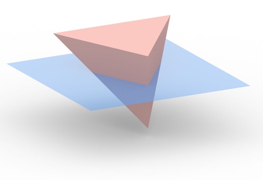
π
Figure 1 Terrain with path π (left); a base surface (center); earth ( ) and and air ( ) (right).
to be constructed from nothing more than an outline: a closed path (loop) on the surface of
the terrain. This outline need not be a contour: its elevation may vary along the outline.
For example, suppose that linear features (ridges, rivulets) or paths (hikers’ tracks) on a
terrain are to be clustered for further analysis. One could project the paths onto the xy-plane
and use an existing polyline similarity measure, like the Hausdorff distance, Fréchet distance,
or area in between. However, such measures do not take into account that there is relief
between the paths: two straight, parallel paths on a flat terrain may be considered more
similar than two paths with the same distance in the projection, but with a ridge in between.
Hence the volume of the terrain between the paths might be a better indicator of similarity.
Consider a second example from landslide susceptibility analysis. Here several factors
play a role, which can be described by geological, hydrological, land cover, and morphological
variables [17]. Thanks to LiDAR and SRTM, many morphological features can be assessed
automatically, without a human visiting the area in question. For example, the volume of
earth on a slope, rising above a certain region (mapping unit [3]), can be estimated via
methods as discussed in this paper and subsequently analyzed for risk of detachment.
Our input is a terrain and an outline, such as the concatenation of two paths or the
outline of a region. We wish to compute a meaningful 2D base surface induced by the outline
so that we can determine a volume of earth above it. In other words, we start with a (1D)
outline, and define a (2D) base surface to compute a (3D) volume (see Fig. 1). A given
outline may also enclose a significant dent, so there could be air below the base surface and
above the terrain surface. In some applications the volume of this air may be relevant. Hence,
we will consider not only the earth above a base surface but also the air below it.
In prior work, we proposed several options to define meaningful base surfaces from an
outline [20]. In this paper we extend our earlier work in two ways. First, we show how to
actually compute the base surfaces and the corresponding volumes from an outline, that
is, we describe algorithms that realize our earlier definitions. Second, we experimentally
compare the proposed surface options for the two aforementioned application examples:
similarity of paths on terrains and landslide susceptibility analysis.
Results and organization. Our input consists of a two-dimensional surface T embedded in
three-dimensional space, representing a terrain, and an outline π, or two paths π1 and π2
that share their endpoints but are otherwise disjoint. In Section 2 we review the options for
base surfaces which we proposed in prior work [20]. We first describe three possibilities for
the most basic of surfaces, namely planes, and argue how to place them optimally. Second,
we consider three options for more general base surfaces which do contain π, or π1 and π2
(which usually cannot be the case with planes). In Section 3 we describe how to compute the
base surfaces as well as the volumes of earth and air between the input surface T and the
base surfaces. Finally, in Section 4 we investigate the different plane and surface options
experimentally, using several real-world datasets as well as informative synthetic data. We
observe the results for the different choices and discuss their characteristics, with respect to
both similarity measures (paths) and terrain morphology (landslides).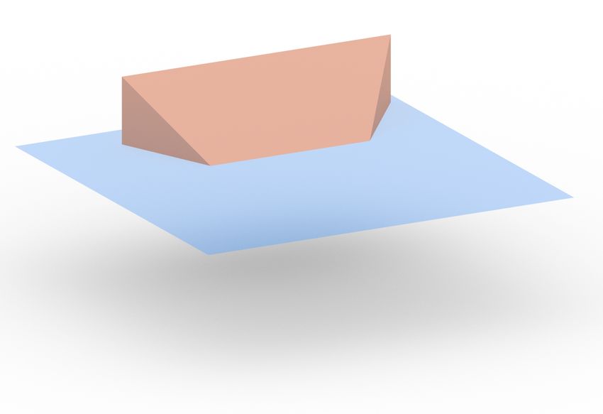
M. van Kreveld, T. Ophelders, W. Sonke, B. Speckmann, and K. Verbeek                                 16:3

Related work. Similarity measures for linear features (shapes) have been considered in a
variety of contexts. Popular geometric measures include the Hausdorff distance, the Fréchet
distance, the area-of-symmetric difference, the Wasserstein distance (Earth Mover’s Distance),
and the turn function distance. Also in GIS, shape similarity measures have been used, for
example, in cartographic generalization. Here a city outline or river shape will be displayed
with less detail on a smaller-scale map, while still capturing the overall shape well. One
needs to measure the similarity between the original shape and the generalized shape to
determine how well the generalization still resembles the original [13, 19]. Furthermore,
similarity measures are used for trajectory similarity [21], landscape ecology [2], (urban)
property analysis [7], spatio-temporal processes [12], and retrieval in spatial databases [15].
There has also been some recent interest in semantic similarity [8, 18], focusing more on
cognitive than on geometric aspects of similarity.
    There is a huge body of research treating landslide susceptibility analysis, surveyed
in [17] (and much earlier in [22]). Morphological factors are an important indicator, but
generally, only simple morphological variables are considered, due to their availability in
GIS [17]. One notable exception is the work by Völker [23] who uses a 6-step approach
utilizing tension surfaces fitted over nearby profiles to reconstruct the ocean floor prior to a
submarine landslide. His method strongly relies on the assumption that the terrain before
the landslide at the position of the landslide is similar to the surrounding area. As such
Völker’s methodology does not apply to the predictive analysis of morphological features
for landslide risk assessment. To analyze unstable landforms like escarpments or features in
poised position [14], we need more advanced terrain shape analysis tools, and we hope that
volumes from outlines can contribute to these developments.

 2     Preliminaries

We review the options for base surfaces induced by an outline which we proposed in earlier
work [20]. Specifically, we describe three linear surfaces (planes) and three general surfaces.
    The horizontal averaging plane (HAP) is the horizontal plane whose elevation is the
average of the elevations of the outline. It minimizes the sum-of-squared vertical distances
from the outline to the plane, over all horizontal planes. The regression plane (RP) is the
(non-horizontal) plane that minimizes the sum-of-squared vertical distances from the outline
to the plane. As a third plane choice, we consider the horizontal plane z = c that minimizes
the sum of absolute differences: p∈π | zp − c | dp. We refer to this plane as the minimizing
                                   R

horizontal plane (MHP); it is located at the median height of π. These planes are – within
the outline – typically partly above and partly below the surface. So we can measure the
volume of earth above and of air below the plane.
    General base surfaces can be of various types. For example, we could use a constrained
Delaunay triangulation on the vertically projected outline and lift it to 3D, similar to the
construction of a triangulated irregular terrain from contour lines. Alternatively, we could
use a minimum tension surface or a minimum curvature surface. However, neither of these
choices is particularly well motivated by our intended applications; we feel that a minimum
area surface (MAS) is a more natural choice. For example, in the context of landslide risk
assessment, a minimum area surface as a base surface represents the case where the area,
and thus the friction between the moving and not moving earth, is minimized.
    The four base surfaces described so far can be used both for a single outline and for
two paths. We next describe a choice of base surface that applies only to two paths. This
surface readily lends itself to measure the similarity between the two paths in a manner
which takes the volume of the relief between them into account. Specifically, the so-called

                                                                                                   GIScience 2021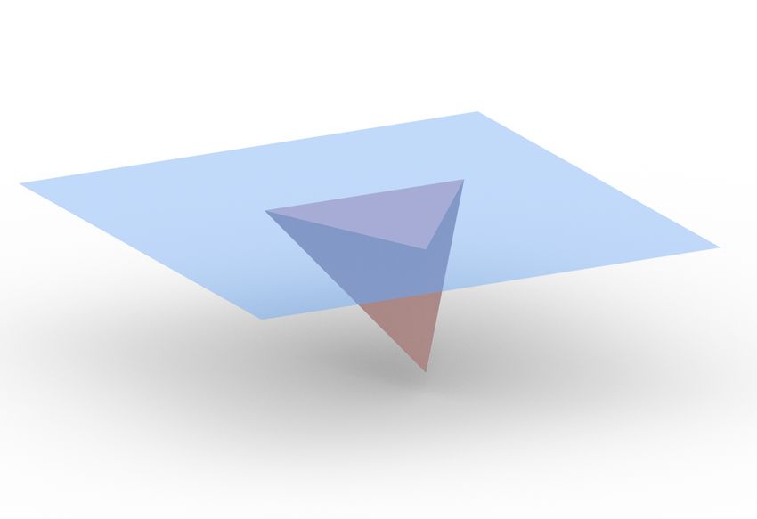
16:4   Volume from Outlines on Terrains

                                        π10                                              π10
             s0                                               s0

                                                     t0                                               t0
           (a)               π20                           (b)                π20

          Figure 2 (a) A monotone isotopy illustrated by intermediate paths of the morph between π10
       and π20 . (b) Two transverse curves of this isotopy. The transverse curve at parameter 0 is simply s0
       and the transverse curve at parameter 1 is t0 , the projections of s and t (taken from [20]).

       water flow surface (WFS) models the ease with which one path can morph into the other.
       It is motivated by morphological processes shaping channels in braided rivers [5, 11]. The
       WFS models the minimum amount of earth that must be removed for a path to change
       its course from π1 to π2 . The WFS cannot be symmetric, for example, if π1 lies further
       uphill than π2 , and is hence defined by an ordered pair (π1 , π2 ). Note that the volume-based
       distance function implied by the WFS is not a metric.
          The transformation from π1 into π2 is essentially a morph. Such a morph should be
       smooth and should not “double-back” on itself, that is, it should be a monotone isotopy (see
       Fig. 2(a)) in the 2D plane, morphing between the 2D projections π10 and π20 of π1 and π2 .
       To construct the surface we need to assign suitable elevations to the points on the paths in
       the morph between π10 and π20 . We can view the curves π10 , π20 , and the ones in between in
       the morph, as parametrized curves where at parameter 0 we are at the common start s0 ,
       and at parameter 1 we are at the common end t0 (see Fig. 2(b)). Points that occur at the
       same parameter form transverse curves. We now choose the WFS to be the surface on or
       below the terrain T such that a monotone isotopy exists for which all transverse curves are
       monotonically decreasing, and among these, the one that has the smallest volume between T
       and the WFS. A more extensive description and motivation can be found in [20].
           We illustrate the difference between the WFS and the RP by a simple example (see
       Fig. 3). Assume that paths π1 and π2 lie in a plane, which is the RP for these paths. The RP
       gives a volume above it and below T that is the whole bump above the plane (see Fig. 3(b)).
       The WFS lies higher and defines a smaller volume, namely the volume of the bump above the
       saddle point (see Fig. 3(c)). Hence, a sloped terrain with some roughness between π1 and π2 ,
       but no local maxima, gives a volume of 0 between T and the WFS. The RP would give some
       volume based on the summed volumes of the roughness spots above the regression plane.
       The WFS distance for the example in Fig. 3(d) is the volume between T and a horizontal
       plane through s and t on one side of the valley.

                  (a)                         (b)                   (c)                        (d)

          Figure 3 (a) A sloped hill with transverse paths. (b) Removing parts by the RP. (c) Removing
       parts by the WFS (above the saddle point) (d) A valley with longitudinal paths (from [20]).
M. van Kreveld, T. Ophelders, W. Sonke, B. Speckmann, and K. Verbeek                                  16:5

   As noted, the WFS is asymmetric: exchanging the roles of π1 and π2 leads to a different
base surface and a different measured volume. Our last base surface is a symmetric version of
the WFS which is again defined for an outline. To define the symmetric flow surface (SFS)
we consider paths on or below T from any point p on or below T inside the outline π to the
outline π. The SFS is the 2D boundary of the union of all points p for which there is a path
on or below T which monotonically increases towards the 1D boundary π. Since these paths
can choose any point on π as their destinations, instead of only a specific part (π1 or π2 ), the
SFS always bounds less volume than the WFS. The SFS is the same as the WFS in Fig. 3(c),
but bounds a volume of 0 in Fig. 3(d), unlike any of the other base surfaces we described.

 3     Computing base surfaces and volumes

In this section we describe how to compute the base surfaces as well as the volumes of earth
and air between the input surface T and the base surfaces. Recall that our input consists
of a two-dimensional surface T , representing a terrain, and an outline π, or two paths π1
and π2 that share their endpoints but are otherwise disjoint. For all base surfaces but WFS,
we first concatenate π1 and π2 into an outline π. We assume that we can model T as a
height function h : R2 → R that maps a geographic position (x, y) to its corresponding height
value. We further assume that T is represented by a TIN, that is, the terrain model consists
of vertices and edges forming triangles, where every vertex v has a position and a height
value associated with it, and heights are interpolated linearly over edges and triangles. The
outline π by extension is a simple polygonal boundary that lies on the terrain surface. Our
methods apply to other elevation models than TINs, such as DEMs and spline surfaces, but
some adaptations are needed.

Computing base surfaces. Computing the planes HAP, RP, and MHP from the input is
straightforward. We interpret the vertices of the outline π as 3D points, and compute these
planes with standard methods.
    The base surfaces MAS, WFS, and SFS are functions B : R2 → R. For ease of computation,
we assume that each base surface B is also represented by a TIN, and the projection onto the
(x, y)-plane coincides with that of T . In other words, B has the same vertices as T , but the
heights of these vertices may differ from those in T . The minimal area surface (MAS) cannot
be represented exactly by a TIN because the surface is curved, but we believe that using the
same TIN as T provides an approximation that is comparable to how well T approximates
the real-world terrain. Computing an approximation to the MAS is computationally intensive.
For a given outline π, we start with a surface based on a weighted average of the vertex
elevations defining the outline π (or π1 and π2 ); the weight for a vertex is proportional to
1/d2 where d is the distance to that vertex. We further optimize using gradient descent, until
a (local) minimum is reached. This is our approximation of the MAS.
    For WFS or SFS, the base surface often overlaps with the terrain T , except where locally
maximal parts are cut off by a horizontal plane at the elevation of a saddle. The boundary of
the base surface uses vertices on the contour line of the saddle. We can therefore represent
these base surfaces implicitly (but still exactly), using annotations in the original terrain T .
To know at which saddles inside π (or π1 ∪ π2 ) we need to trace the contour lines, we use a
highest path tree which represents all highest paths towards π or π1 . A highest path tree can
be computed efficiently [1, 11].

                                                                                                    GIScience 2021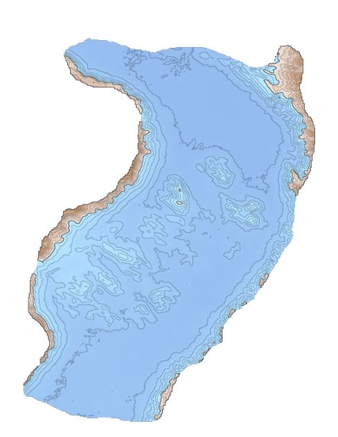
16:6   Volume from Outlines on Terrains

       Computing volumes. The volume V of earth above the base surface B for an outline π, for
       all six base surfaces, is defined as follows (see Fig. 1):
                    Z
           V (π) =     max 0, h(x, y) − B(x, y) dx dy.                                     (1)

                     D

       Here D is the domain of the function that corresponds to the part of the terrain inside π.
       Alternatively, we can measure the volume V 0 of air below the base surface:
                   Z
          V (π) =
            0
                       max 0, B(x, y) − h(x, y) dx dy.                                       (2)

                     D

       We now describe how we can compute these integrals in practice. For that we use the fact
       that the terrain T is represented as a TIN.
           Assuming that T and B share the same TIN (with different heights), we can compute the
       integral in Equation 1 (or similarly, in Equation 2) as follows. We split up the domain D
       into triangles corresponding to the projections of the triangles in T onto the (x, y)-plane.
       For each such triangular domain, the function h(x, y) − B(x, y) is linear by the definition of
       a TIN, and this function is completely determined by the values of h(x, y) − B(x, y) at the
       vertices of the triangle. Let h1 ≤ h2 ≤ h3 be the corresponding values at the vertices of the
       triangle. We will simply refer to these values as height.
           To compute the integral for a single triangular domain, we need two basic building blocks,
       namely the volume of a prism and the volume of a pyramid:

          Vprism = Ah;              Vpyramid = Ah/3,

       where A is the area of the base of the prism/pyramid and h is the height of the prism/pyramid.
       We now consider several cases. First of all, we assume that h3 > 0 (otherwise the integral
       is 0) and that h1 < 0 (otherwise we can simply add a prism with height h1 to the volume).
       The following cases remain:
       Case 1 (h1 < h2 < h3 ): We cut up the triangle into two triangles by cutting it at height h2 .
           Note that for the two resulting triangles, two vertices share the same height; we can use
           Case 2, 3 or 4 to compute their corresponding volumes separately.
       Case 2 (0 = h1 = h2 < h3 ): The remaining volume is a pyramid.
       Case 3 (h1 = h2 < 0 < h3 ): We cut the triangle at height 0 and end up in Case 2.
       Case 4 (h1 < 0 < h2 = h3 ): We add a pyramid on top of the triangle to form a prism.
           We then compute the volume of the prism with height h3 and subtract the volume of
           the pyramid, except for the part of the pyramid that is below height 0 (see Fig. 4). The
           volume of the tip of this pyramid can be computed as in Case 3.
       To compute the integral in Equation 1 for the WFS or the SFS, we take a similar approach,
       using the implicit representation of B in T . The computations can be simplified because
       WFS and SFS are never above T .

                               h3
                h2

                                        =                −                 +

                          h1

          Figure 4 Computing the volume below the triangle and above the zero plane (blue) in Case 4.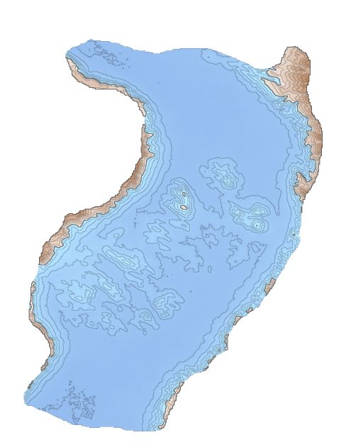
M. van Kreveld, T. Ophelders, W. Sonke, B. Speckmann, and K. Verbeek                                 16:7

 4      Experiments
We implemented our methods and investigated the different plane and surface options
experimentally, using several real-world datasets as well as informative synthetic data. In
this section we observe the results for the different choices of base surfaces and discuss their
characteristics, with respect to both similarity measures (Section 4.1) and terrain morphology
(Section 4.2).

4.1     Volume-based path similarity on terrains
We used two extracts from the world-wide SRTM elevation dataset: one of the area around
Mont Blanc on the border of France and Italy, and one of Grampians National Park, Australia.
Both extracts were taken from the void-filled SRTM data sets produced by CIAT [9]. In
both datasets we manually drew three input paths π1 , π2 , and π3 that are of interest. In the
Mont Blanc dataset we drew two paths π1 and π3 through valleys, and one path π2 that
goes higher along the mountain (but not over the peak, see Fig. 5(a)). In the Grampians
dataset we drew two paths π1 and π3 along mountain ridges, and one path π2 in the valley
between (see Fig. 5(b)). We also constructed a small set of synthetic datasets that clearly
illustrate the features of our base surfaces and the associated volumes.
    To measure the volume-based similarity between two paths, we define the distance
between them with respect to a particular base surface as the volume of earth and possibly
air between this base surface and the terrain. The distances (the computed volumes) are
shown in Tables 1, 2, and 3; we express all values in 109 m3 .

Mont Blanc dataset. In Table 1 we show the results for the Mont Blanc dataset. The first
column shows the distance between π1 and π3 , the second column the distance between π1
and π2 , and the third column the distance between π2 and π3 . Every row in the table shows
the result for a different base surface. For each combination of base surface and pair of paths
we show: (1) a grayscale figure showing the height of the base surface, (2) a color figure
showing the amount of earth (brown) or air (blue) measured with respect to the base surface,
and (3) the corresponding volumes measured for earth ( ) and air ( ), if applicable.

                                                                   t

                                      t

                                                             π1
                  π1       π2
                                                                       π2   π3

                                 π3

                       s                     (a)         s                       (b)

     Figure 5 Datasets and paths: (a) Mont Blanc. (b) Grampians.

                                                                                                   GIScience 2021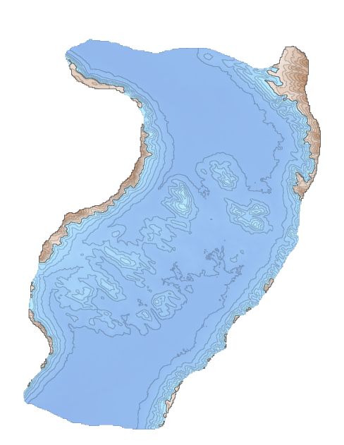
16:8   Volume from Outlines on Terrains

          Table 1 Mt. Blanc, distances between (π1 , π3 ), (π1 , π2 ), and (π2 , π3 ), earth (   ) and air (   ).

        Area (108 m2 )

        Projected         6.627                          3.508                          3.119
        Actual            6.742                          3.568                          3.174

        HAP

                                   314.10 24.77                   25.77 33.72                    160.60 9.07

        RP

                                   297.87 8.32                    29.60 16.39                    158.58 6.23

        MHP

                                   305.13 26.85                   27.73 31.21                    169.97 7.47

        MAS

                                   310.59 0.90                    9.07    10.94                  143.35 0.64

        WFS
        →
                                      117.92                          15.34                          22.36

        WFS
        ←
                                      17.32                           0.64                           16.69

        SFS

                                      17.29                           0.60                           16.69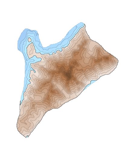
M. van Kreveld, T. Ophelders, W. Sonke, B. Speckmann, and K. Verbeek                                16:9

    Since both paths π1 and π3 are in valleys, we expect the base surfaces to separate a lot
of earth and not much air. All of the HAP, RP, MHP, and MAS distances appear to have
this property, although the horizontal planes separate more air than intuitively desirable.
The WFS separates much less of the earth (especially in one direction), and the same holds
naturally for the SFS. However, these distances still appear to capture the most important
parts of the mountain (at least the WFS (→) does). These distances are expected to measure
less, as they are more conservative and more closely follow the input terrain.
    If we consider the distances between π1 and π2 , then we expect to measure less earth, and
relatively more air. This indeed appears to be the case for all distances that also measure
air. Also for WFS and SFS the distances clearly appear to measure less earth. There is
an interesting difference to notice here between the RP and MAS distances: because the
RP is restricted to be a plane, it is well below the higher parts of π2 , thus the RP distance
measures much more earth than the MAS distance.
    Finally, since the peak is contained between π2 and π3 , we expect our distances to measure
more earth (relative to projected area) than between π1 and π2 . Again, the HAP, RP, MHP,
and MAS distances clearly capture this. The same holds for the WFS (←) and SFS distances.
As WFS (→) essentially just separates earth that needs to be removed to travel monotonically
from π1 to π2 (capturing the part of the mountain left from π2 ) and from π2 to π3 (capturing
only the peak to the right of π2 ), it is not surprising that the corresponding distances are
similar.
    It is further interesting that the WFS (→) distance between π1 and π2 (capturing the
part of the mountain left from π2 ) and the WFS (←) distance between π2 and π3 (capturing
the part of the mountain right from π2 ) are roughly the same. We would expect the latter
to be higher, since that part contains the peak of the mountain. This discrepancy can be
explained by the fact that the path π3 is higher than the path π1 . Finally, note that for most
distances, the amount of earth measured between π1 and π3 is higher than the the sum of
the amounts of earth measured between π1 and π2 and between π2 and π3 . This is desired
behavior, as the paths π1 and π3 are both in different valleys and thus very different. It also
directly implies that these distances do not satisfy the triangle inequality.

Grampians dataset. In Table 2 we show the results for the Grampians dataset, in the same
structure as for the Mont Blanc dataset. Since the paths π1 and π3 enclose a large valley, we
expect to measure a lot of air in this dataset. This indeed appears to be the case for the
distances based on HAP, RP, MHP, MAS. Especially the MAS is good at not separating
any unnecessary earth near the paths π1 and π3 . However, none of these distances capture
the small hills inside the valley. These hills are measured by the WFS distances, but they
also measure some extra volume near the paths π1 and π3 . The SFS distance picks up the
volume of the hills inside the valley only.
    Since the path π2 goes through the valley, we expect the distances between π1 and π2
to capture much less air than between π1 and π3 . This is indeed the case for the HAP, RP,
MHP, and MAS distances. However, the MHP distance appears to capture very little air
and more earth than expected. This is due to the fact that the MHP uses the median height
of the paths. Since more than half of π1 ∪ π2 lies in the valley, the base surface MHP also
lies in the valley, thus separating a large amount of earth. Further, as before, the HAP, RP,
MHP, and MAS distances do not measure the hills inside the valley. This volume is measured
by the WFS (→) distance. The WFS (←) distance also measures it, but it measures a
significant amount of extra volume near π1 . Finally, the SFS distance again nicely captures
the volume of the small hills in the valley.

                                                                                                  GIScience 2021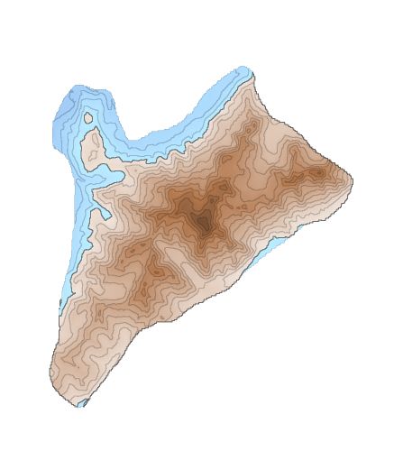
16:10   Volume from Outlines on Terrains

           Table 2 Grampians, distances between (π1 , π3 ), (π1 , π2 ), and (π2 , π3 ), earth (   ) and air (   ).

         Area (108 m2 )

         Projected         6.627                          3.508                          3.119
         Actual            6.742                          3.568                          3.174

         HAP

                                    6.78    167.63                 7.15    47.24                   9.75    40.16

         RP

                                    6.05    168.24                 6.65    38.56                   4.56    45.96

         MHP

                                    4.97    191.45                 26.33 4.43                      21.57 7.61

         MAS

                                    0.66    173.19                 0.65    48.35                   1.10    33.49

         WFS
         →
                                        23.55                          1.89                           21.40

         WFS
         ←
                                        23.84                          21.59                           1.39

         SFS

                                        3.26                           1.87                            1.37
M. van Kreveld, T. Ophelders, W. Sonke, B. Speckmann, and K. Verbeek 16:11
For the distances between π2 and π3 we expect similar results as between π1 and π2 , and
indeed the HAP, RP, MHP, and MAS distances appear to give similar values. We also clearly
see the asymmetry of the WFS distance, where the WFS (→) and WFS (←) distances have
switched roles compared to the values between π1 and π2 . The SFS distance again nicely
captures the volume of the small hills in the valley.
Like in the Mont Blanc dataset, we see that the amount of air measured between π1
and π3 is more than the sum of the amounts of air measured between π1 and π2 and between
π2 and π3 . Again, this is desired behavior. This dataset also illustrates the usefulness of the
WFS and SFS distances. In particular, from the SFS distance we can see that the volume
of the hills in the valley to the left of π2 is more than to the right of π2 , which is almost
impossible to see from the HAP, RP, MHP, and MAS distances.
Synthetic datasets. In Table 3 we show the results for the synthetic datasets. The synthetic
datasets are (1) a hill, (2) a slope, (3) a set of small hills on a slope, and (4) a valley where
the two paths start in the valley, go up different sides of the valley, and then end up down in
the valley again.
For the first dataset with the hill, all distances clearly measure the volume of the hill.
The distances measure small amounts of air, but these amounts are clearly insignificant.
For the slope dataset there are clear differences. Depending on what behavior is desired,
different distances should be chosen. If the paths should be considered to be different, then
one should simply measure the area/projected area between the paths, or use the HAP or
MHP distances. Because the HAP and MHP distances use horizontal planes as base surface,
they cannot capture the slope and must measure significant volumes of both earth and air.
The WFS distance is useful for a situation where going up implies more distance than going
down. However, given our motivation of contextual volume-based distances, these paths
should have distance zero, and this is indeed measured by the RP, MAS,1 and SFS distances.
The third synthetic dataset also contains a slope, so the HAP and MHP distances give
similar results as for the second synthetic dataset. Also, the WFS distance again demonstrates
its inherent asymmetry. The remaining distances (based on the RP, MAS, and SFS) all
capture the small hills on the slope. SFS is generally more conservative in measuring the
earth volume.
The fourth synthetic dataset shows some interesting differences between the distances.
The HAP, RP, MHP, and MAS distances all capture the air in the valley between the high
parts of the paths. The HAP and RP distances also capture some earth volume near the
high parts of the paths. The WFS distances capture how much “effort” it costs to go from
one path to the other, where only moving up requires effort. The effort here is measured
as the amount of earth that needs to be removed to eliminate this effort. Finally, the SFS
distance measures the amount of effort needed for the two paths to come together.
4.2 Volumes from outlines for landslide risk analysis
We next analyze how our base surfaces and the corresponding volumes may contribute to
landslide risk analysis. To that end, we consider a part of real-world terrain (see Fig. 6) that
has been identified as high risk for landslides according to the deep-seated landslide suscepti-
bility map for California, USA, created by the California Department of Conservation [24].
1
The MAS distances are not exactly zero. This is a consequence of approximating a minimum area
surface; the real minimum area surface should follow the slope and result in a distance of zero.
GIScience 202116:12 Volume from Outlines on Terrains
Table 3 Synthetic data, distances between π1 and π2 , earth ( ) and air ( ).
HAP
29.91 0.08 15.63 15.63 11.08 9.56 5.59 46.85
RP
29.91 0.08 0 0 3.80 2.29 5.59 46.85
MHP
30.10 0.05 15.63 15.63 12.67 8.28 0 82.52
MAS
29.67 0.00 0.36 0.39 3.56 1.75 0.06 37.05
WFS
↓
28.54 15.63 1.29 29.66
WFS
↑
28.54 0 11.82 29.66
SFS
28.54 0 1.05 0
Specifically, we consider a part of terrain along the California coastline close to Highway 1
(near the mouth of Russian river), which has been assigned the highest risk class X among
eight different classes. The classification is based on the slope of the terrain and the soil
type, but does not take volume or other aspects of the shape of the terrain into account.M. van Kreveld, T. Ophelders, W. Sonke, B. Speckmann, and K. Verbeek 16:13
1
2 4
3
(a) (b) (c)
Figure 6 Regions used in our landslide analysis: (a) overview map; (b) part of the deep-seated
landslide susceptibility map for California (image from CGS Map Sheet 58 [24]); (c) the four regions.
For a more fine-grained analysis of landslide risk, it is relevant to measure the amount
of soil (that is, volume) that may slide and where this soil may be deposited. We believe
that (some of) our volumes from base surfaces can contribute to such analysis. To show
that, we consider four equal-size ellipse-shaped regions of the terrain that all have the same
risk class X in the deep-seated landslide susceptibility map, but contain parts of the terrain
with different morphology (see Fig. 6). Specifically, Region 1 contains a convex ridge with
relatively high plan curvature, Region 2 contains a valley with negative plan curvature, and
Regions 3 and 4 are flatter, but Region 3 borders the valley of Region 2, whereas Region 4
does not. We computed three volumes on the region outlines, using the RP, MAS, and SFS.
Note that the volumes from horizontal planes are not meaningful (the terrain is sloped for
all regions), and that the WFS requires two paths instead of a single outline, so we did not
include them in this analysis. The results are shown in Table 4.
We can immediately see that the SFS volume is small. This is to be expected: the SFS
is designed for similarity in the context of water flow, and therefore only separates volume
around local maxima (as they impede water flow). Since all regions contain sloped terrain
without significant local maxima, the SFS always separates near-zero volumes. The volumes
based on the RP and MAS are similar. If we interpret the outline of a region as the boundary
of a potential landslide, then indeed we would expect to measure a high volume of earth
for the ridge (Region 1). On the other hand, we measure very little earth for the valley
(Region 2), as expected. However, the volume of air is very high. This indicates that a
large volume of soil can be deposited in this region, but the region does not contribute much
soil to any landslide. For Regions 3 and 4, which are flatter than Region 1, the RP and
MAS indeed separate less earth volume than for Region 1. The earth volume for Region 3 is
somewhat higher than for Region 4, likely because Region 3 borders the valley of Region 2,
and hence one part of the outline of Region 3 drops down steeper there. Also note that,
purely based on morphology, the outline of Region 4 is not likely the border of a potential
landslide, as the profile of the terrain is not changing much across the outline. However,
geological, hydrological, and land use factors may indicate otherwise.
Considering the (minor) difference between the RP and MAS volumes, we see that the
volumes for the MAS are somewhat “cleaner”. For example, the MAS separates no air volume
for the ridge (Region 1), as one would expect, whereas the RP separates a small volume of
air. The reason for this is that the MAS can completely follow the terrain at the outline, and
the RP, which is a flat plane, cannot. This results in small amounts of air and earth volume
close to the outline unnecessarily being added to the total earth and air volumes separated
by the RP. These amounts become larger as the outline becomes more irregular (less flat).
However, we can see that these added amounts are relatively small and do not change the
volumes significantly. Given the fact that the RP can be computed much faster than the
MAS, the RP volume might be preferable if there is no need for high precision.
GIScience 202116:14 Volume from Outlines on Terrains
Table 4 Landslides, volume measurements in 105 m3 for the four areas, earth ( ) and air ( ).
1 2 3 4
RP
20.25 0.09 2.55 18.36 8.95 0.88 7.62 0.74
(angle 8.3°) (angle 8.6°) (angle 10.5°) (angle 8.8°)
MAS
22.28 0.00 2.04 19.69 10.09 0.71 6.06 0.24
SFS
0.01 0.00 0.00 0.00
5 Conclusion
We studied the problem of computing a volume of terrain based on a given outline. After
reviewing six possible base surfaces, we showed how to compute them and how to determine
the volume between a base surface and the terrain. We highlighted two use cases, namely
volume-based similarity and landslide risk assessment, and performed experiments related
to both of them. The experiments revealed properties of the different volume computation
models so that practitioners can easily select the most suitable one for their application.
Summarizing, we have demonstrated that computing terrain volume based on an outline is a
useful type of terrain analysis. We presented various options to do so, including the required
algorithms, and reported on extensive comparative experiments.
References
1 Mark de Berg and Marc van Kreveld. Trekking in the Alps without freezing or getting tired.
Algorithmica, 18(3):306–323, 1997.
2 Enrico Feoli and Vincenzo Zuccarello. Spatial pattern of ecological processes: the role of
similarity in GIS applications for landscape analysis. In Manfred Fischer, Henk J. Scholten,
and David Unwin, editors, Spatial Analytical Perspectives on GIS, pages 175–185. Taylor &
Francis, 1996.
3 Fausto Guzzetti, Alberto Carrara, Mauro Cardinali, and Paola Reichenbach. Landslide hazard
evaluation: a review of current techniques and their application in a multi-scale study, Central
Italy. Geomorphology, 31(1-4):181–216, 1999.
4 L. A. M. Hendriks, H. Leummens, A. Stein, and P. de Bruijn. Use of soft data in a GIS
to improve estimation of the volume of contaminated soil. Water, Air, and Soil Pollution,
101(1-4):217–234, 1998.M. van Kreveld, T. Ophelders, W. Sonke, B. Speckmann, and K. Verbeek 16:15
5 Matthew Hiatt, Willem Sonke, Elisabeth A. Addink, Wout M. van Dijk, Marc van Kreveld, Tim
Ophelders, Kevin Verbeek, Joyce Vlaming, Bettina Speckmann, and Maarten G. Kleinhans.
Geometry and topology of estuary and braided river channel networks automatically extracted
from topographic data. Journal of Geophysical Research: Earth Surface, 125(1), 2020.
6 Jeffrey Hollister and W. Bryan Milstead. Using GIS to estimate lake volume from limited
data. Lake and Reservoir Management, 26(3):194–199, 2010.
7 Alec Holt. Spatial similarity and GIS: the grouping of spatial kinds. In Proceedings of the
11th Annual Colloquium of the Spatial Information Research Center (SIRC05), pages 241–250,
1999.
8 Krzysztof Janowicz, Martin Raubal, Angela Schwering, and Werner Kuhn. Semantic similarity
measurement and geospatial applications. Transactions in GIS, 12(6):651–659, 2008.
9 A. Jarvis, H.I. Reuter, A. Nelson, and E. Guevara. Hole-filled seamless SRTM data V4, 2008.
URL: http://srtm.csi.cgiar.org.
10 A. Keutterling and A. Thomas. Monitoring glacier elevation and volume changes with digital
photogrammetry and GIS at Gepatschferner glacier, Austria. International Journal of Remote
Sensing, 27(19):4371–4380, 2006.
11 Maarten Kleinhans, Marc van Kreveld, Tim Ophelders, Willem Sonke, Bettina Speckmann,
and Kevin Verbeek. Computing Representative Networks for Braided Rivers. In Proceedings
of the 33rd International Symposium on Computational Geometry (SoCG 2017), volume 77 of
LIPIcs, pages 48:1–48:16, 2017.
12 John McIntosh and May Yuan. Assessing similarity of geographic processes and events.
Transactions in GIS, 9(2):223–245, 2005.
13 Robert B. McMaster and K. Stuart Shea. Generalization in Digital Cartography. Association
of American Geographers, 1992.
14 Colin W. Mitchell. Terrain Evaluation. Routledge, 2014.
15 Giorgos Mountrakis, Peggy Agouris, and Anthony Stefanidis. Similarity learning in GIS:
an overview of definitions, prerequisites and challenges. In Spatial Databases: Technologies,
Techniques and Trends, pages 294–321. IGI Global, 2005.
16 Pascal Peduzzi, Christian Herold, and Walter Claudio Silverio Torres. Assessing high altitude
glacier thickness, volume and area changes using field, GIS and remote sensing techniques:
the case of Nevado Coropuna (Peru). Cryosphere, 4(3):313–323, 2010.
17 Paola Reichenbach, Mauro Rossi, Bruce D Malamud, Monika Mihir, and Fausto Guzzetti. A
review of statistically-based landslide susceptibility models. Earth-Science Reviews, 180:60–91,
2018.
18 Angela Schwering. Approaches to semantic similarity measurement for geo-spatial data: A
survey. Transactions in GIS, 12(1):5–29, 2008.
19 K. Stuart Shea and Robert B. McMaster. Cartographic generalization in a digital environment:
When and how to generalize. In Proceedings of Auto-Carto 9, pages 56–67, 1989.
20 Willem Sonke, Marc van Kreveld, Tim Ophelders, Bettina Speckmann, and Kevin Verbeek.
Volume-based similarity of linear features on terrains. In Proceedings of the 26th ACM
SIGSPATIAL International Conference on Advances in Geographic Information Systems,
pages 444–447, 2018.
21 Kevin Toohey and Matt Duckham. Trajectory similarity measures. Sigspatial Special, 7(1):43–
50, 2015.
22 David J. Varnes. Landslide Hazard Zonation: a review of principles and practice. Number 3
in Natural Hazards. United Nations, 1984.
23 David Julius Völker. A simple and efficient GIS tool for volume calculations of submarine
landslides. Geo-Marine Letters, 30(5):541–547, 2010.
24 C. J. Wills, F. G. Perez, and C. I. Gutierrez. Susceptibility to deep-seated landslides in
California, 2011. California Geological Survey, Map Sheet 58.
GIScience 2021You can also read