WASHU EPIGENOME BROWSER - 2018 epigenomegateway.wustl.edu
←
→
Page content transcription
If your browser does not render page correctly, please read the page content below
WASHU EPIGENOME BROWSER
           2018
 epigenomegateway.wustl.edu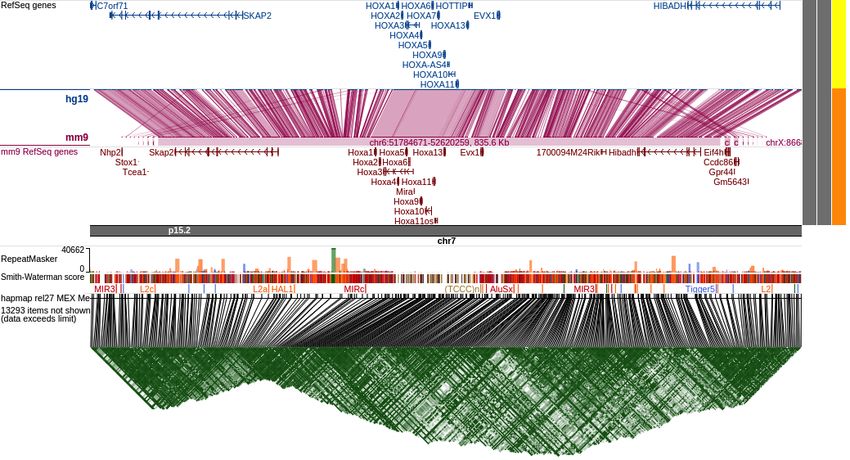
BROWSER MAP
                               3 14 15 16 17 18 19 20 21 22 23 24

                                                                        5
                               1                                    2   4

                           8

                           9

                          10

                          12

                           6

                          11

                           7

                          13

Key
1     = Go to this page number to learn about the browser feature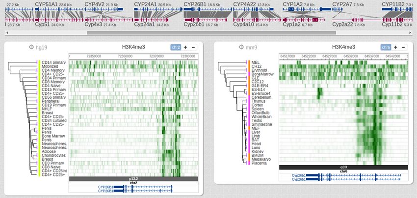
TABLE OF CONTENTS

             1.   Navigation
 BROWSER     2.   Tracks
 FEATURES    3.   Apps
             4.   Metadata
             5.   Metadata Heatmap

             6.   Genes
             7.   Repetitive Elements
             8.   Numerical Tracks
 BROWSER     9.   Matplots
  TRACKS     10. MethylC Track
             11. Genome Comparison
             12. Long-Range Interaction
             13. SNPs and LD

             14. File Upload
   DATA      15. Datahub
MANAGEMENT   16. Screenshot
             17. Session

             18. Gene & Region Set View
             19. Split Panel
  APPS       20. Juxtaposition
    &        21. Genome Snapshot
FUNCTIONS    22. Find Orthologs
             23. Scatter Plot
             24. Gene Plot
             25. Roadmap EpiGenome Browser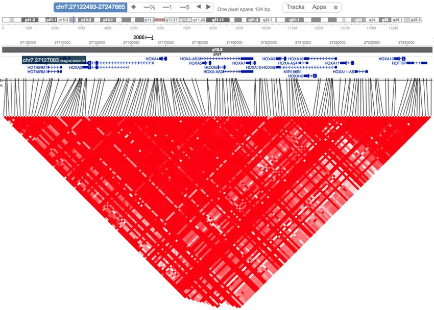
1                          Browser Features: Navigation

                                     Click to zoom in.
                                                    Click to zoom out.
                      Click to show options.
                                                                         Click to scroll.

                                                                          Chromosome
                                                                          ideogram.
                                         Scale
                                                                          Coordinate ruler.

                                                                            Drag on
                                                                             ruler to
                                                                            zoom in.
               Drag on track
                 to scroll
                                                                          Chromosome
                                                                          ideogram of region.

    Enter coordinates to jump to a region.       Enter a gene name to jump to a gene.

    Coordinate string can be one of:             Multiple gene models may be shown for
                                                 a gene. Choose one gene model to
       1.   chr9:1234-5678 a region.             jump to its location.
       2.   chr9:123456 a single base.
       3.   chr9 a chromosome to jump
            to the middle of that
            chromosome.
       4.   1234-5678 coordinates
            without a chromosome name
            to jump to this region on the
            current chromosome.

    Enter the reference SNP cluster ID
    (rsID) to jump to a specific SNP.

     At fine resolution, the
     chromosome ideogram is
     replaced by the DNA sequence.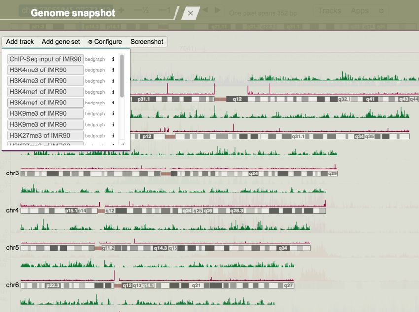
Browser Features: Tracks                                           2

   A browser track is a visualization of a dataset along a genome. Examples of browser
   tracks include gene model annotation tracks and RNA-seq expression tracks.

              Tracks        Click to find browser tracks.

                                                   Click the box labeled with total track count
                                                   to access all available experimental assay
                                                   tracks from the interactive facet table.

        Search for tracks by
        keywords. Join multiple
        keywords with “AND“.

         Access annotation tracks such
         as genes.
                                                   The numbers indicate the tracks
                                                   available for each sample+assay
                                                   combination (green) and the tracks that
                                                   are currently shown in the browser (red).
                                                   Click a table cell to show a list of
                                                   available tracks for a sample+assay
                                                   combination.

                                                   Show available public track hubs to
 Click a button to submit a custom track.          load tracks from projects including
                                                   Roadmap Epigenomics Project and
                                                   ENCODE.
    8

    6       11         12

   15

Click “Reference human epigenomes from
Roadmap Epigenomics Consortium” and then
the “Load” button to load the Roadmap
Epigenomics dataset.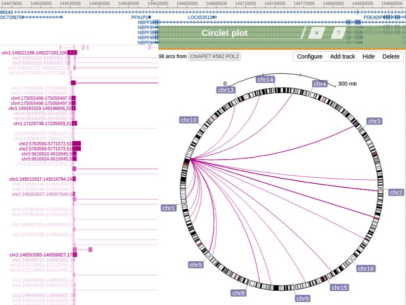
3
1                            Browser Features: Apps

    A browser app is a self-contained program for executing a specific task. Examples of
    browser apps include uploading files and taking screenshots.

                                     Apps       Click to find browser apps.

                                                        Find apps by name.
                                                        Apps will appear as you type.

                                                        Show all apps.

                                                        Recently used apps.

                                                   14

                                                  18

                                                  21

                                                  23          Frequently used apps.

                                                  19

                                                  17

                                                  16

                 Apps usually appear as transparent panels on top of the
                 browser and are used in the context of browser visualization.
                 You never have to leave the browser to use an app.

                 Drag the app name
                 banner to move the panel.              Close this app.   Get help on this app.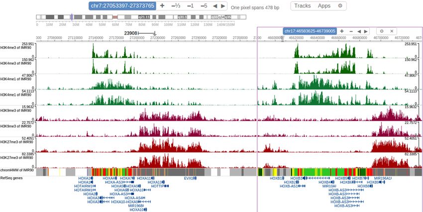
Browser Features: Metadata                                        4

                                            Metadata are vocabularies for
                                            annotating tracks with experimental and
                                            sample information. Terms in a
                                            vocabulary are organized in a
                                            hierarchical structure. The same
                                            vocabulary can be used across
                                            datasets to facilitate data integration.

To load metadata vocabularies
available for the human genome,
load the public datahub for the
Roadmap Epigenomics Project. The
metadata annotation for a track can
be viewed by right-clicking a track
and selecting “Information."

                                                                          Internal
                                                                          metadata

To view loaded metadata vocabularies,
right-click on the metadata heatmap
header, then select “Add metadata terms”.
                                          Metadata
                                  5
                                       vocabularies.

Once a metadata vocabulary has been
loaded, its terms can be searched by
keyword. Results include the term id for
each found term. The term id can be
used to annotate tracks in a datahub.

             Learn more about how to define metadata vocabularies and annotate
Wiki         tracks at http://wiki.wubrowse.org/Metadata.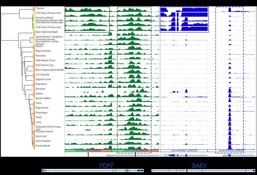
5                Browser Features: Metadata Heatmap

             A metadata heatmap with two
             metadata terms.

                                                          Tracks 1, 2, and 3 share the
                                                          same “sample” attribute
Track 1                                                   (IMR90 cells) and thus share
                                                          the same color.
                                                          Tracks 1, 2, and 3 are each
Track 2                                                   annotated by a different “assay”
                                                          attribute (H3K4me3, H3K4me1,
                                                          H3K27me3) and thus are
Track 3                                                   colored differently.

                                                          Track 4 is not annotated by
Track 4                                                   “sample” or “assay” attributes
                                                          so is shown in gray.

                                                          Chromosome ideogram.

                                                          Track 5 is below the
Track 5                                                   chromosome ideogram and
                                                          thus is not shown in the
                                                          metadata heatmap.

    To add or remove a track from the metadata heatmap, drag the track name above or
    below the chromosome ideogram.

    To search for new terms to be added to the
    metadata heatmap, right-click the term name and
    then open the Metadata term finder app by
    clicking “Add metadata terms."

                                                 The source metadata vocabulary. 4

                                                 Click to show this term in the heatmap.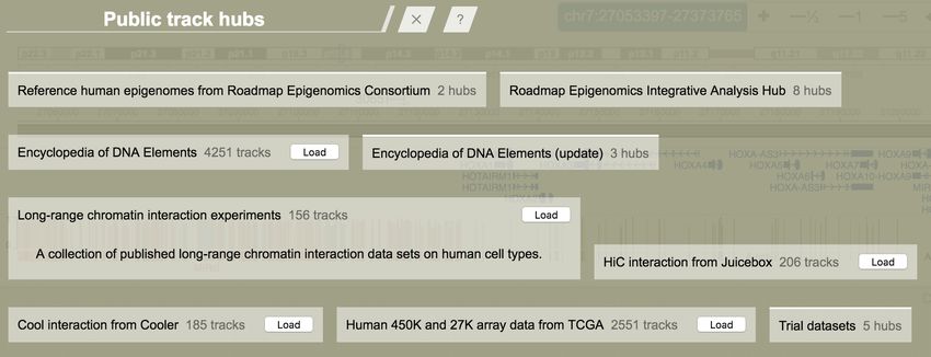
Browser Tracks: Genes                                            6

                       UTR.       Exon.      Intron. Arrows indicate direction of transcription.

                                                                              Transcription
                                                                              start site.

   Gene symbol.                                                             Link to NCBI
                                                                            Nucleotide database.

                                                                         Gene body coordinates,
    Gene name.                                                           orientation, and length.

  Coordinates of
exons and UTRs.

   The human RefSeq gene track for HOXA3 is shown above. The tooltip bubble
   displays information on the HOXA3 gene.

   Multiple gene tracks are usually available
   for a genome. To find other gene tracks,
   go to “Tracks” > “Annotation tracks”
   >“Genes” or search by keyword “gene” in
   “Tracks."

   When a gene is partially visible in the
   browser, click this gene to display the
   entire gene model in the tooltip bubble.
   The visible section is marked by a yellow
   box.

   Right-click on the                Display modes.
   gene track (and any
   other tracks) for the   Configure rendering style.
   configuration
   menu.                       20 View only genes.
                                    Show metadata.

                                          Link to Wiki.

                   The gene track is based on the “hammock” track format, which can be
                   displayed as a custom track.
     Wiki
                   Learn more at http://wiki.wubrowse.org/Hammock.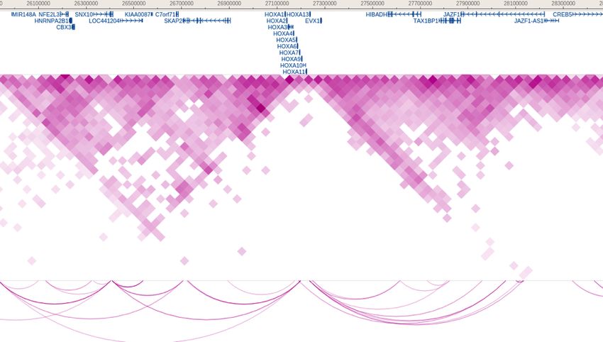
7                    Browser Tracks: Repetitive Elements

    The RepeatMasker and RepeatMasker slim tracks show all repetitive elements in the
    genome. Repetitive elements and transposons are predicted by the RepeatMasker
    software (http://www.repeatmasker.org/).

    To add the RepeatMasker track, go to “Tracks” >
    “Annotation tracks” > “RepeatMasker” >
    “RepeatMasker“. The track is also available as
    RepeatMasker slim, a simplified version of the
    RepeatMasker track.

    Full mode          Elements are shown as boxes, transparency reflects the 1-divergence% score of
                       each element. More transparent elements have greater divergence.

    Bar plot mode      Elements are packed tightly into a single row with bars on
                       top indicating 1-divergence% scores.

The elements are colored by class. To view                The user can choose which type of score to
the list of classes, right-click the                      show for the repetitive elements using the
RepeatMasker track and click “Configure.”                 configuration menu.

Hover over a specific element to display the              The user can also choose to show elements
element’s score, class, name, and genomic                 from a specific class or family in the
position.                                                 Annotation tracks menu.

                    The repetitive element track is based on the “hammock” track format.
       Wiki         Learn more at http://wiki.wubrowse.org/Hammock.
Browser Tracks: Numerical Tracks 8
A numerical track displays a series of quantitative values along the genome as a
highly customizable graph. When the track height is small, the track is shown as a
heatmap, otherwise it is shown as a bar plot.
Bar plot (track height ≥ 20 pixels) Heatmap (track height < 20 pixels)
Positive and negative values are
rendered using different colors.
The default y-axis scale is an automatic
scale which can be changed into a fixed
or percentile scale using the configuration
menu. Bars with values beyond a set
threshold are indicated with a different
color on the peaks.
Bar plot shape can be smoothed using the configuration menu.
A background can be applied to bar plots to distinguish regions with no data from
those with low data values.
No background With background
Missing values are labelled as “No data” on
the tooltip for bedGraph format tracks
(not applicable for bigWig format tracks).
Learn more about the supported numerical track formats
Wiki bedGraph (http://wiki.wubrowse.org/bedgraph) and
bigWig (http://wiki.wubrowse.org/bigwig).9 Browser Tracks: Matplots
A matplot (also called a line plot) displays multiple numerical tracks on the same X
and Y axes to easily compare datasets. Data is plotted as curves instead of bar plots.
Matplots can be created while browsing:
Method 1:
1. Hold shift and click on track names
to select multiple numerical tracks.
(Track names will be highlighted in
yellow.)
2. Right-click on the selected tracks
and select “Apply matplot."
Method 2:
Right-click on a colored box in the metadata
heatmap and select “Apply matplot” to
convert a group of tracks sharing the same
metadata attributes into a matplot.
Colors of member tracks in a matplot can be
individually configured using the configuration
menu.
To cancel a matplot, right-click on the track and
select “Cancel matplot." The matplot will be
replaced by individually displayed member
tracks.
Matplots can be defined in datahub.
Wiki Learn more at http://wiki.wubrowse.org/matplot.Browser Tracks: MethylC Track 10
The methylC track1 is designed to display DNA methylation data from whole-genome
bisulfite sequencing experiments. It distinguishes cytosine methylation levels (as bar
plots) on separate strands and in different sequence contexts and integrates
sequencing read depth (as curves) as a measure of confidence.
The color legend for a methylC track can be viewed
using its configuration menu. All colors are
configurable by clicking on the color boxes.
To filter methylation data by read depth, in the configuration menu, select “Filter by
read depth," enter a threshold, and click “Apply."
No filtering Filtered by read depth value 5
To combine the forward and reverse strands, in the configuration menu, select
“Combine two strands."
To scale the methylation level bar plots by read depth, in the configuration menu,
select “Scale bar height by read depth." The y-axis value will now represent the
read depth.
Wiki Learn more about MethylC tracks at http://wiki.wubrowse.org/MethylC_track.
1Zhou X, et al., Bioinformatics 30, 2206-2207 (2014)11 Browser Tracks: Genome Comparison
The genome comparison track visualizes pairwise alignments of two genomes allowing
for comparison at fine (base pair) or large (megabase) scale. Alignment is unbiased with
gaps in both the query and target genomes.
To add the genome comparison track,
go to “Tracks” > “Annotation tracks” >
“Genome comparison."
Many pre-built genome comparison
tracks are available.
Annotation tracks for either species can
now be loaded using the tracks panel.
Human HOXC10. 3 bp gap on the human genome. Human genome
as target.
sequence
|||||||||||
alignment
Mouse Hoxc10. 2 bp gap on the Mouse genome
mouse genome. as query.
At 10 bp/pixel resolution, the browser will transition from individual alignment blocks to
a joined alignment block.
Individual alignment blocks.
Joined alignment block.
Complex genome rearrangements can be visualized by observing synteny blocks.
Wiki Learn more at http://wiki.wubrowse.org/Genome_alignment.Browser Tracks: Long-Range Interactions 12
Long-range chromatin interaction experiments can be accessed through public track hubs1.
Human HOXA gene cluster.
Hi-C data from IMR90 cells shown as ChIA-PET data from K562 cells
a heatmap. shown as arcs.
Highlights:
1. Supports pairwise chromatin interaction results from Hi-C, 5C, and ChIA-PET.
2. Multiple display modes: heatmaps, arcs, and joined-boxes (full display).
3. Visualizes interactions from distant regions and different chromosomes.
4. The Circlet view visualizes global interactions.
Hi-C data from
IMR90 cells shown
as joined-boxes.
Wiki Learn more at http://wiki.wubrowse.org/Long-range.
1Zhou X, et al., Nature Methods 10, 375-376 (2013)13 Browser Tracks: SNPs and LD
Human dbSNP release 137.
Human HapMap LD
Han Chinese (CHB).
SNP and LD annotation tracks are available for human genomes. By default, the LD
scoring system is D’. The correlation coefficient (R square) or LOD can be displayed
using the configuration menu.
These tracks can be found in the “Population variation” group of the annotation track
panel. To search for a SNP, type the reference SNP cluster ID (rsID) into the search
bar and click “Find SNP." SNPs are colored by class.
The SNP and LD tracks are based on the “hammock” track format.
Wiki Learn more at http://wiki.wubrowse.org/Hammock.Data Management: File Upload 14
Use the File Upload app to upload data
from a text file.
Click the “Choose files(s)” button to
select one or more unzipped text files
from the computer for upload.
Selected files appear as
boxes.
To prepare a file for upload:
1. Click the “Setup” button.
2. Inspect the content of the first 10 lines.
3. Select the appropriate file format.
4. Click “add as Track” to load this file as a custom track or
click “add as Set” to load this file as a gene set. The gene
set option is limited to 100 items per set.15 Data Management: Datahub
A datahub is a collection of data from multiple sources.
An example datahub.
[
# this hub contains only one track
{
type:"bedgraph",
url:"http://vizhub.wustl.edu/hubSample/hg19/GSM432686.gz",
name:"my track",
mode:"show",
colorpositive:"#ff33cc",
height:50,
},
]
Highlights:
1. Batch uploading of many tracks at the same time.
2. Custom track information is preserved in a datahub.
3. Tracks in a datahub can come from different servers.
4. Track rendering style can be customized.
5. Tracks can be annotated with metadata.
A datahub is written in JSON text. The JSON content of a datahub can be
validated by the browser. Search for the “Validate datahub” app to run validation.
Use the datahub app to upload a datahub to the browser.
A datahub file can be either hosted on the Web or saved locally.
If the datahub is hosted on the Web, it can be referenced by the browser through
the URL parameter. In this way, you can bookmark the parameterized browser
link for quick reference or sharing.
http://epigenomegateway.wustl.edu/browser/?genome=hg19&datahub=http://
vizhub.wustl.edu/hubSample/hg19/hub.json
Dissecting the browser URL parameters.
genome
browser URL ?genome= &datahub= datahub URL
identifier
Learn more about datahubs (http://wiki.wubrowse.org/Datahub) and
Wiki URL parameters (http://wiki.wubrowse.org/URL_parameter).Data Management: Screenshot 16
Use the Screenshot app in the Apps menu to save
images of the current genomic view.
The “Screenshot” app will convert the browser contents to an SVG file. The SVG
file is a high-quality vector-based graphics file. In addition, a PDF file will also be
created.
To take a screenshot, click the “Take screenshot” button. Links to both the SVG
and PDF files will be displayed.
Click either link and the file will be shown on the browser. From either page
you can save the file to your computer.17 Data Management: Session
Use the Session app in the Apps menu to save the
current browser status, including tracks, view range,
and customization, for later viewing.
To save a session, click the “Save” button. Enter a
name for this session (optional). A link to the saved
session will appear. Alternatively, the user can
download the session as a JSON datahub file.
Multiple session names
can be saved under one
session ID.
A link is generated for each session name.
A session can be recovered in three ways:
1. Save the generated link and simply use this link to reload the session.
2. Upload a saved JSON datahub file by clicking the “Upload” button in the “Sessions”
app.
3. Copy the unique session ID and paste this into the “Retrieve” box in the “Sessions”
app.
Sessions and datahubs only record information about tracks; they do not save actual track data.
If the track file has been moved, the browser won’t be able to recover that track from the
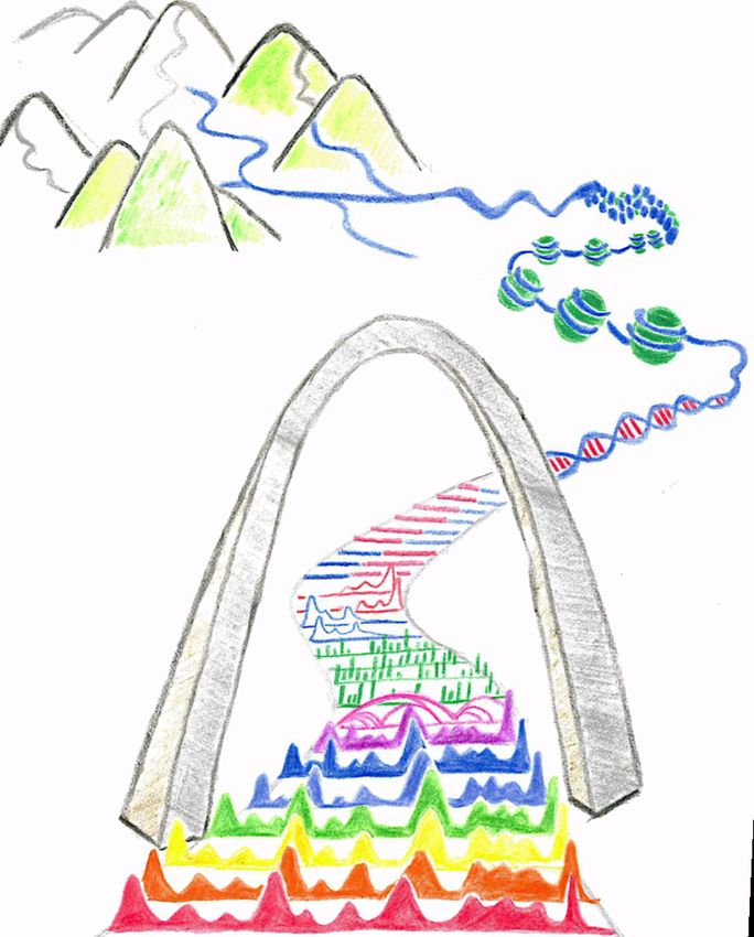
session or datahub.Apps: Gene & Region Set View 18
Use the Gene & region set app to show track data over a set of genes or regions. The
“Gene & region set” app enables track data to be displayed over regions that are not
adjacent on a chromosome or even on different chromosomes.
Red: 2.5 KB Green: 2.5 KB
downstream of TSS. upstream of TSS.
Middle: gene transcription start site (TSS).
The user can create a set of genes or regions of
interest.
Gene and region sets can be submitted in three
ways:
1. By pasting a list of gene names or genomic
coordinates in the “Gene & region set” app.
2. By file upload in the “Gene & region set” app.
3. By using predefined KEGG pathways.
The user can specify custom flanking regions (up to
5 KB on each side) surrounding the gene
transcriptional start sites to focus on the gene
promoters.
“Gene set view” can be applied to see all regions in
one browser view. To quit the gene set view, click
the pink button next to the zoom buttons near the top
of the browser.19 Apps: Split Panel
Use the Split panel app to “split” the browser panel in two. The order of the tracks
remains the same in both of the panels, but the panels can be separately scrolled and
zoomed. This allows the user to easily explore data patterns of the same set of tracks
across two different genomic locations.
Main panel navigation buttons. Split panel navigation buttons.
HOXA HOXB
gene cluster gene cluster
Main panel Split panel
When splitting the browser panel, the browser inserts a
blank panel to the right of the existing panel.
Click the “SELECT VIEW RANGE”
button to choose a view range for
the new panel.Features: Juxtaposition 20
Use the juxtaposition function to focus on data over a subset of the genome.
After juxtaposing on RefSeq genes, intergenic regions are hidden, and only data
over gene bodies are shown. When running juxtaposition, the browser can be
zoomed and scrolled as normal. The juxtaposition function is applicable for other
types of positional annotation data in addition to genes.
To run juxtaposition, right-click on a gene or annotation track and click
“Juxtapose." To quit the juxtaposition view, right-click on any gene or annotation
track and click “Undo juxtaposition."
Normal view Genomic view with intergenic regions included.
Juxtaposition view Genomic view with intergenic regions removed.
In the following example, juxtaposition reveals enhancer signatures (H3K4me1)
over several LTR elements that are otherwise hard to see.21 Apps: Genome Snapshot
Use the Genome snapshot app in the Apps menu to visualize
the genome-wide profile for numerical tracks over all
chromosomes.
Numerical tracks from the browser can be added to the genome snapshot using the “Add
track” button. Above, H3K4me1 and H3K4me3 of IMR90 cells are shown. Just like browser
tracks, track styles can be customized when the user right clicks. The global view can be
changed using the “Configure” button. Lastly, a snapshot of all chromosomes can be captured
and saved using the “Screenshot” button.Apps: Find Orthologs 22
Use the Find orthologs app to identify highly similar genomic regions from the
query genome for a set of target genomic regions based on the information in a
genome-comparison track.
To find orthologs:
1. Display a genome-comparison track by
selecting “Tracks” > “Annotation Tracks” >
“Genome comparison”.
2. Create a gene set for the target genome.
3. Send this gene set to the “Find orthologs” app.
4. Click the “find orthologs” button.
5. View or export the result.
25
For each target region, the most similar region is found from the query genome
based on the data in the genome alignment track. In the resulting output, the
target genome regions are ranked by length in descending order. Each pair of
aligned regions is graphically rendered.
Target gene name. Line width
Target genome gene model.
indicates relative region length.
Sequence
alignment.
Target genome coordinate. Query genome gene name, gene
model, and coordinate.23 Apps: Scatter Plot
Use the Scatter plot app in the Apps menu to assess the
relationship between two numerical tracks over a gene set.
Choose a pre-made gene set. Choose two
numerical tracks for the x- and y- axes and
click “SUBMIT."
Anti-correlation between
H3K4me3 (active mark) and
H3K9me3 (repressive mark)
in human IMR90 cells over a
list of regions.
The plot is interactive. Mouse
over each datapoint for
information.
Click a datapoint to show its
corresponding region in the
browser.
Customization options.
In making the scatter plot, the average value over each item in the gene set is
calculated for both numerical tracks.Apps: Gene Plot 24
Use the Gene plot app to explore the data variation and distribution of a numerical
track with respect to a group of genes or regions of interest. The gene set needs to be
loaded using the “Gene & region set” app before using the “Gene plot" app. Search
for the “Gene plot” app in the Apps menu.
Choose a gene set.
Select the data to be plotted.
Four plots (box plot, matplot, gene part
plot, and clustering) are available, and
each is fully customizable.
Plots can be rendered in either R or
Google Charts.
Gene transcription start sites.
2.5 KB upstream of TSS. 2.5 KB downstream of TSS.
The above boxplot shows the IMR90 H3K4me3 signal distribution over 5 KB regions
centered on the transcription start site of 100 random human genes. Data from each
region is evenly summarized into 100 data points, and a boxplot is shown over each
summary point to indicate the data distribution. Outliers are hidden in the boxplot.
Individual curves for each item. Profile over gene features. Hierarchical clustering.25 Roadmap EpiGenome Browser
The Roadmap EpiGenome Browser1 is built on top of the WashU EpiGenome
Browser to serve as a point-of-access to explore and analyze comprehensive
epigenomics data generated by the Roadmap Project.
Highlights:
1. Access tens of thousands of epigenomic assays with a few clicks.
2. Applies real-time data clustering to reveal cell type-specificity of
epigenetic marks.
3. Reveals covariations of epigenomic profiles and gene expression.
4. Integrates datasets from Roadmap Epigenomics and ENCODE projects.
5. Supports cross-species epigenome comparison (human and mouse).
Visit the browser at: http://epigenomegateway.wustl.edu/browser/roadmap
Select a genome (human hg19 and/or
mouse mm9) and click “Load” to continue.
The browser starts loading information on the
samples.
Click the Navigation box to choose a view range.
Select an assay type to launch the
browser.
Browser
options.
Navigation
options.
Hierarchical
clustering. High H3K4me3
appears over the
Sample names. CHRNA7 promoter
in tissues including
brain, but not
blood cells.
RefSeq genes.
1Zhou X, et al., Nature Biotechnology 33, 345-346 (2015)Roadmap EpiGenome Browser 25
1 Epigenetic annotation of genetic variants
Multiple sclerosis-associated noncoding SNPs are annotated using epigenomic and
expression data. rs307896 marks an enhancer common across all displayed samples,
whereas rs756699 is located in an enhancer specific to immune cells.
2 Cross-species epigenome comparison
Human and mouse epigenomes can be compared over orthologous regions.
Human and mouse homologous genes found by the “Find orthologs" app. 22
Click an alignment to show epigenomes over the two regions.
Human Mouse
epigenome epigenome
samples samples
over the over the
human gene mouse geneNotes
Notes
Everything can be found at
                     epigenomegateway.wustl.edu

      REFERENCES
        1. Zhou X, et al., Nature Methods 8, 989-990 (2011)
        2. Zhou X & Wang T, Current Protocols in Bioinformatics Unit 10.10
           (2012)
        3. Zhou X, et al., Nature Methods 10, 375-376 (2013)
        4. Zhou X, et al., Bioinformatics 30, 2206-2207 (2014)
        5. Zhou X, et al., Nature Biotechnology 33, 345-346 (2015)
        6. He Yu, et al., Bioinformatics 33, 3268-3275 (2017)

      FUNDING
           NIH 5U01ES017154, NIH R01ES024992, NIH R01HG007175,
            NIH R01HG007354, NIDA DA027995, RSG-14-049-01-DMC,
            U01CA200060, U24ES026699, U01HG009391

      LATEST DEVELOPMENT
            Google+: epigenomegateway.wustl.edu/+
            Facebook: epigenomegateway.wustl.edu/fb
            Twitter: @wuepgg

      SUPPORT
                         epigenomegateway.wustl.edu/support/

      CONTACT US Lab: wang.wustl.edu
                      Browser Developers: Xin Zhou, Daofeng Li, Deepak Purushotham, and Silas Hsu
Booklet Authors: Renee Sears, Vasavi Sundaram, Rebecca Lowdon, Erica Pehrsson, and Nicole Rockweiler
                                             Principal Investigators: Joseph Costello and Ting Wang
                                                                              Cover art: Ting Wang
V: 1/2018                                        Copyright © WashU EpiGenome Browser 2010-2018
You can also read