An Investigation into Chemical Kinetics and the Arrhenius Equation for Activation Energy

An Investigation into Chemical Kinetics and
 the Arrhenius Equation for Activation Energy

 11 PAGES

IB CANDIDATE CODE:
SUBMISSION DATE: 29.01.2021

1

TABLE OF CONTENTS

Introduction ......................................................................................................................................................................... 2
Equipment and chemicals .............................................................................................................................................. 4
 Chemicals.......................................................................................................................................................................... 4
 Equipment ........................................................................................................................................................................ 4
Method.................................................................................................................................................................................... 4
 Risk assessment ............................................................................................................................................................. 4
 Procedure ......................................................................................................................................................................... 4
Raw Data ................................................................................................................................................................................ 6
Processed data .................................................................................................................................................................... 6
 Calculating initial rate ................................................................................................................................................. 6
 Calculating the activation energy ........................................................................................................................... 9
Conclusion .......................................................................................................................................................................... 11
Evaluation .......................................................................................................................................................................... 11
Appendix A – Raw data ................................................................................................................................................. 13
Appendix B – Processed data ..................................................................................................................................... 14

2

INTRODUCTION
The idea for this investigation came about when I was trying to open a bottle of soda. It had been
tossed around inside my bag, so it fused up when I tried to open it. A friend of mine told me that if
I opened it slowly, the foam would be released over a longer period, leading to less spilling. This
led me to investigate something regarding rate. After learning about the rate of reaction in class, I
decided that I wanted to investigate the relationship between temperature and rate. But why
might this be a relevant field of investigation in the scientific community? Fritz Haber discovered
by looking at rates that the speed of the reaction depended largely on the fact that the triple bond
in nitrogen is really hard to break. He and his assistant were able to develop catalysts which
allowed this process to occur at a much faster rate. 1 This developed into the Haber process, which
is used to produce fertilizer today, almost 100 years after its discovery. 2

The mathematical model for the Haber process was developed by a Swedish scientist named
Arrhenius. He was both a physicist and chemist, and his work is closely linked to the Maxwell-
Boltzmann energy distribution for different temperatures (Figure 1 3 ). This is what we call
collision theory which states that with a higher temperature, the number of molecules that have
kinetic energy above the activation energy, will be greater. This should in theory make the
reaction proceed faster, meaning that the rate would be greater. In this investigation, I wish to
look at the relationship between initial rate and temperature, as well as experimentally determine
the Arrhenius Activation energy (Ea) for the reaction between sodium carbonate and dilute
hydrochloric acid.

 Figure 1. Maxwell - Boltzmann energy distribution.

In order to test the effect of temperature on the initial rate of reaction, I found a chemical reaction
that produces a gas to measure the rate at which the gas is produced. Sodium carbonate reacts
with hydrochloric acid, carbonic acid is produced.
 Na2 CO3 (aq) + HCl (aq) → 2 NaCl (aq) + H2 CO3
Since carbonic acid is unstable, it decomposes as shown in the reaction below:
 H2 CO3 → H2 O + CO2 (g)

1 “Chemistry - Rates of Reaction,” University of Birmingham, last modified 2020, accessed January 27,
2021, https://www.birmingham.ac.uk/teachers/study-resources/stem/chemistry/reaction-rates.aspx.
2 Wikipedia Contributors, “Haber Process,” Wikipedia (Wikimedia Foundation, January 20, 2021), last

modified January 20, 2021, accessed January 28, 2021, https://en.wikipedia.org/wiki/Haber_process.
3 Horrocks, Mathew. “Reaction Rates, Temperature and Catalysis.” 4college.Co.Uk. Last modified 2020.

Accessed October 24, 2020. http://www.4college.co.uk/a/aa/rate.php.

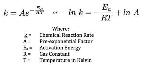
3

The final reaction will therefore be:
 Na2 CO3 (aq) + HCl (aq) → 2 NaCl (aq) + H2 O (l) + CO2 (g)
Hence, we can measure the rate at which carbon dioxide gas is produced. This would allow us to
calculate the initial rate, as well as calculating the activation energy for this reaction.

 Figure 2. Linearization of Arrhenius Equation.

To find the activation energy, I first need to find the rate constant. As seen in Figure 2 4, if I plot
 1
the natural logarithm of the rate constant on the y-axis, and on the x-axis, the gradient of the
 
graph will be − where R is the gas constant. This means that the activation energy is the
 
gradient multiplied by -8.31. The rate constant can be calculated from the rate law. The rate law
in its power form is as follows:
 rate = k ∗ [A]n ∗ [B]m
Where k is the rate constant, [A] and [B] are the concentration of reactants, and n and m are rate
orders. The law of mass action predicts that a reaction in a dilute soliton, the rate only depends on
the concentration of the reactants, raised to the power of their stoichiometric coefficients. 5 Since
the concentration of sodium carbonate is 1.0, the rate order n does not matter. The stoichiometric
coefficient for hydrochloric acid is 2, and its molarity is 2.0. Hence, the rate constant is given by
the following equation:
 Initial rate Initial rate
 k = =
 2.02 4
Research questions: What is the relationship between temperature and initial rate? What is the
activation energy for the reaction between sodium carbonate and hydrochloric acid?
Independent variable: Temperature
Dependent variable: Rate of reaction
Research hypothesis: The initial rate of reaction will be greater at higher temperatures.

4 “Arrhenius Equation and Stability Studies,” Blogspot.com, last modified 2012, accessed January 29, 2021,
http://stabilitystudies.blogspot.com/2012/06/arrhenius-equation-and-stability.html.
5 “Physical Chemistry,” Google Books, last modified 2013, accessed January 27, 2021,

https://books.google.no/books?id=lk2PzH9LmS8C&dq=isbn:0716787598&hl=no&sa=X&ved=2ahUKEwi
Yz_S8wr_uAhVuAhAIHZerDMgQ6AEwAHoECAAQAg.

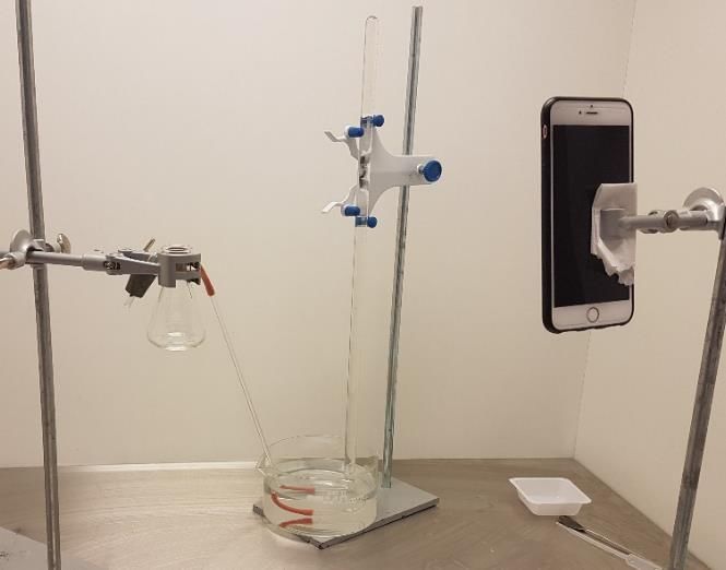
4

EQUIPMENT AND CHEMICALS
Equipment Chemicals
 - Digital scale ± .001 g
 - Sodium carbonate,
 - Thermometer ± .05 oC
 Na2CO3 (s). Dissolved in water to
 - 2x Pipette 10.000 ml ± .020 ml
 make a solution with
 - 3x Beaker 100 ml
 1.00 ± 0.08 mol dm-3.
 - Beaker 300 ml ± 5 ml (for solution)
 - Beaker >400ml (for waste) - Dilute hydrochloric acid,
 - 2x Vertically standing arms HCl (aq), 2.0 ± 0.1 mol dm-3.
 - Clamp
 - Erlenmeyer flask 50 ml
 - Rubber bung (sized to fit the Erlenmeyer flask)
 - Small tube
 - Graduated measuring cylinder 50.00 ml ± 0.05 ml
 - Suitable clamp for the measuring cylinder
 - Wide jar to create water trough
 - Video capturing device
 - Water bath
 - Magnetic stirrer

METHOD
Risk assessment
Sodium carbonate, Na2CO3, is a base and causes serious irritation if it comes in contact with the
eyes. To account for this, I wore glasses and I avoided touching my face when handling the
chemicals.
Hydrochloric acid, HCl, is a strong acid and can cause skin corrosion and irritation. To prevent
this, I made sure that the acid only persisted in the beaker in which it was heated and cooled in,
as well as in the pipette. I also washed my hands after handling the acid.
The chemicals were not heated directly but rather placed into separate beakers that were placed
into the water bath. The water bath was not heated with a hotplate for other trials than the one
with the highest temperature, and the lower temperatures were rather placed into hot tap water.
The fridge used to cool the solutions was a fridge designated to the lab, only containing chemicals
and no food.
Once all trials for all temperatures were complete, the beaker with sodium chloride was emptied
into a suitable container for chemical waste.

Procedure
Step 1: Initial setup and preparation of chemicals
I started by setting up the equipment as shown in Figure 3. The main takeaways are that the
Erlenmeyer flask has to be higher in elevation than the bottom measuring cylinder which collects
the gas. This is so that the gas will flow from the flask and into the measuring cylinder, displacing
the water already in it. By doing this, I was able to read the volume of carbon dioxide gas, which
equals the volume of water being displaced.

5

When I was preparing the sodium carbonate solution, I performed several test trials to deduce
which concentration was suitable for my experiment. This was done to make sure that the rate of
the reaction would be neither too big nor too small. The results of my test trials were that 1.00
mol dm-3 sodium carbonate was suitable. In the 300 ml beaker, I prepared 300 ml of solution (an
excess amount of what I needed). This was done by measuring 31.821 g ± 0.001 g sodium
carbonate (Mr (Na2CO3) * 0.3) and dissolving it in 300 ml ± 5 ml of water. I used a magnetic stirrer
to make sure it dissolved fully in the water. By the stoichiometric relation between sodium
carbonate and hydrochloric acid, 1:2, I decided to
use 2.0 mol dm-3 of HCl.
Step 2: Achieving the desired temperatures
Around 50 ml of sodium carbonate solution and
hydrochloric acid were poured into separate 100
ml beakers. These beakers were placed in the
fridge for the coldest temperature, left at room
temperature for the second temperature, and for
the three hottest trials they were heated in the
same water bath. I measured the temperature of
the sodium carbonate. I assume that the
temperature is the same for HCl. When the desired
temperature was reached, the beakers were
removed from the water bath.
 Figure 3. Setup of the experiment. Water bath not
Step 3: Mixing the reactants shown.

After removing the beakers from the water bath, I immediately recorded the temperature of the
sodium carbonate. I used one of the 10.000 ml ± .020 ml pipettes and measured 10.000 ml ± .020
ml sodium carbonate and emptied the pipette into the Erlenmeyer flask. Then I took the other
10.000 ml ± .020 ml pipette and measured 10.000 ml ± .020 ml of hydrochloric acid. When
performing my test trials, I initially took the HCl from the pipette directly into the Erlenmeyer
flask, but when the pipette was empty, and I was going to place the rubber bung, the rate at which
the bubbles were forming had already decreased a lot. Hence, the acid was placed into a beaker in
order to pour it into the Erlenmeyer flask quicker. I continued by pouring the acid into the flask
as quickly as I could without spilling. The rubber bung was placed into the opening of the
Erlenmeyer flask immediately after while making sure the seal was tight. I waited 30 seconds for
the reaction to take place and then ended the trial.
Step 4: Measuring the volume of gas
The production of gas and displacement of water was recorded with the camera on my phone for
each trial. The volume of carbon dioxide gas was read off by looking at the videos and noting down
how much water was displaced after time intervals of 3 seconds. The products left in the
Erlenmeyer flask was poured into a separate waste beaker with a volume of 600 ml. Steps 2
through 4 were repeated three times for 5 different temperatures: T1=10oC, T2=22oC, T3=30oC,
T4=40oC, and T5=50oC.

6

RAW DATA

Table 1. Raw data from temperature 3. T0 is the initial temperature. All the volumes in Table 1 are the volume
of CO2 gas (displaced water) after X seconds.

 Temperature 3 Trial 1 Trial 2 Trial 3 The data set is very spacious (5x3x11).
 T0 in oC (± .05 oC) 31.00 31.80 30.10 Therefore, to save space, I have only included
 the raw data for temperature 3 (Table 1). The
 3s (± .05 ml) 3.60 3.70 3.20 rest can be found in Appendix A. I will use the
 6s (± .05 ml) 9.10 8.50 5.40 data from the three trials with temperature 3
 9s (± .05 ml) 9.60 9.30 6.10 to show my work in calculating the initial rate
 and the activation energy.
 12s (± .05 ml) 10.20 10.00 7.10
 15s (± .05 ml) 10.90 10.50 7.85 A qualitative observation was when the
 reaction proceeded, bubbles were produced.
 18s (± .05 ml) 11.40 11.45 8.30
 This was the carbon dioxide that I attempted
 21s (± .05 ml) 12.00 12.15 8.70 to collect. A fizzling sound was also produced
 24s (± .05 ml) 12.35 12.85 9.70 together with the bubbles.
 27s (± .05 ml) 13.00 13.30 10.40
 30s (± .05 ml) 13.45 14.10 11.00

PROCESSED DATA
Calculating initial rate
To calculate the initial rate for each temperature, I calculated the average initial temperature as
well as the average volume of gas collected after X seconds.
Table 2. Average values for the five temperatures. The uncertainties stated are from the equipment.

 T1 T2 T3 T4 T5
 T0 in oC (± .05 oC) 14.13 21.40 30.97 37.80 51.17
 3s (± .05 ml) 0.00 0.00 0.00 0.00 0.00
 6s (± .05 ml) 5.50 1.02 3.50 3.35 3.33
 9s (± .05 ml) 8.73 3.92 7.70 5.85 11.78
 12s (± .05 ml) 9.68 4.95 8.30 6.22 12.40
 15s (± .05 ml) 10.42 5.53 9.10 6.5 12.77
 18s (± .05 ml) 10.98 6.03 9.80 6.52 13.07
 21s (± .05 ml) 11.60 6.68 10.40 6.67 13.43
 24s (± .05 ml) 12.08 7.30 11.00 6.88 13.77
 27s (± .05 ml) 12.68 7.65 11.60 7.00 13.98
 30s (± .05 ml) 13.40 8.10 12.20 7.15 14.20

7

Data calculations
I made a table in Logger Pro using both manual and calculated columns, so I only had to plot in a
couple of values, instead of all. This made it easier to process the large data set since it involves a
fair number of calculations per temperature. The number of moles of CO2 is calculated from the
ideal gas law.
 pV = nRT
 pV
 n=
 RT
Where p is pressure in Pascal, V is the volume in m3, n is the number of moles, R is the gas constant
and T is the temperature in Kelvin. In my case, V is the volume of CO2 and temperature is the initial
temperature in Kelvin. I have to assume that the pressure in the measuring cylinder follows STP
conditions (100kPa). In the calculations, I have made sure to change the units to fit the equation.
The following shows the calculation for row 2 in Table 3 (page 8, time = 3 seconds).
 pV 105 ∗ 3.50 ∗ 10−6
 n(CO2 produced) = = = .000139 mol (3 s. f. )
 RT 8.31 ∗ (30.97 + 273)
 n(Na2 CO3 remaining) (n(Na2 CO3 initial) − n(CO2 produced))
 c(Na2 CO3 ) = =
 V(Na2 CO3 ) V(Na2 CO3 used)
 n(Na2 CO3 remaining) = n(Na2 CO3 initial) − n(CO2 produced)
 = (1.0mol dm−3 ∗ 10.0ml ∗ 10−3 ) − .000139 = .010 − .000139
 = .00986 (3. s. f)
This is value is stated more accurately than it should. Rounding off all the values mid-calculation
would not yield a good result. Hence, I choose to keep the number of moles with three significant
figures, and not round off anything except the Activation Energy at the end.
 1.0 − .000139
 Concentation after 3s = = .986 mol dm−3
 0.010
Uncertainty calculations
 measurement uncertainty . 05
% uncertainty in temperature = ∗ 100 = ∗ 100 = .16% (2 s. f. )
 measured temperature 30.97
 measuring uncertainty . 05
 % uncertainty in volume = ∗ 100 = ∗ 100 = 1.4% (2 s. f. )
 measured volume 3.50
 (% uncertainty in temperature + % uncertainty in volume)
Abs. uncertainty n(CO2 ) = ∗ n(CO2 )
 100
 (.16% + 1.4%)
 = ∗ .000139 = ± 2.2 ∗ 10−6 mol (2 s. f)
 100
 . 001 5.0 . 020
 % Uncertainty n(Na2 CO3 initial) = ( + + ) ∗ 100 = 1.9% (2 s. f. )
 31.821 300 10.0
 1.9
 Abs. uncertainty n(Na2 CO3 initial) = ∗ (1.0 ∗ 10 ∗ 10−3 ) = ± 1.9 ∗ 10−4 mol (2 s. f. )
 100
 % Uncertainty n(Na2 CO3 remaining)
 (Abs. uncertainty n(Na2 CO3 initial) + abs. uncertainty n(CO2 ))
 = ∗ 100
 n(Na2 CO3 remaining)
 (1.9 ∗ 10−4 + 2.2 ∗ 10−6 )
 = ∗ 100 = 1.9% (2 s. f. )
 . 00986

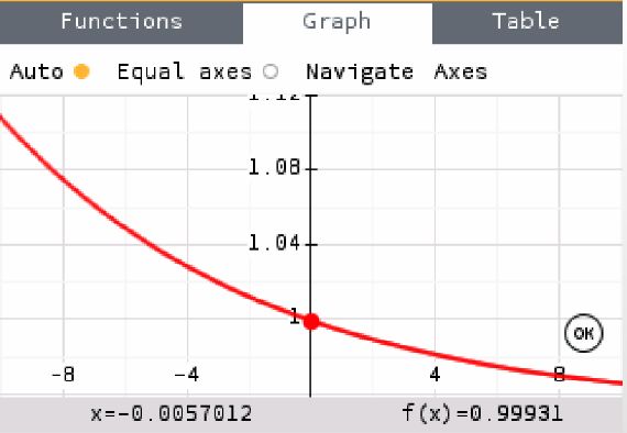
8

 . 020
 % Uncertainty in v(Na2 CO3 used) = ∗ 100 = .20% (2 s. f. )
 10.0
 % Uncertainty in concentration = 1.9% + .20% = 2.1% (1 d. p. )
 2.1%
 Abs. uncertainty in concentration = ∗ 0.986 = ± .021 (2 s. f. )
 100
Table 3. Processed data for T3. Data from Table 2. The columns containing delta (Δ) shows uncertainty with
either percentage or absolute values (as stated in the parentheses). These are needed since the uncertainty in
equipment will affect the calculations later. All uncertainties are rounded to two significant figures. 6

Figure 4. The regression line for data in Table 4, plotting a concentration-time graph for Temperature 3.

The initial rate is given by the rate of change of concentration when time = 0s, which means a
tangent to the graph in Figure 4 at t=0s. I plotted the values from the regression line on a graphing
calculator and found the initial rate (Figure 6). This process was repeated for all five temperatures
and the results can be found in Table 4.

6 Similar tables for T1 through T5 is located in Appendix B.

9

For T2 through T5 the initial rate is increasing when the temperature is higher. This is visualized
in Figure 5, which shows a general increase with higher temperatures. This is not the case for T1.
Since T1 is an outlier it will be discarded for the rest of the calculations. I will discuss this in the
evaluation part of the paper.

Figure 6. Initial rate for Temperature 3. Figure 5. Initial rate and temperatures. Best-fit line without T1.
(dy/dx=-0.0057012)

Calculating the activation energy
Table 4. Processed data for plotting Activation Energy.

To convert the temperature in Celsius to Kelvin I simply added 273 to my value, and since this is
a constant the uncertainty does not play a role, hence the temperature in Kelvin is written as 2
decimal places.
 30.97 + 273 = 303.97 K (2 d. p. )
 . 05
 % uncertainty of temperature = ∗ 100 = .16% (2 s. f. )
 30.97
1
 
 in Kelvin is needed to plot the activation energy.

 1 1
 = = .0032898 −1 (5 s. f. )
 T 303.97
This is displayed as 5 significant figures since that is the least number in the calculation. The initial
rate and its uncertainties are from Figure 6 and Table 3, respectively. Since the theoretical
uncertainty at t=0s is infinitely big (division by zero), I use the average uncertainty for the rest of
my domain. This turns out to be 2.2% for all five temperatures. The percentage uncertainty of k is
the same as the percentage uncertainty in the initial rate.
 2.2
 Abs. uncertainty in k = ∗ 1.4 ∗ 10−3 = ± 3.1 ∗ 10−5 (2 s. f. )
 100

10

When taking the natural logarithm of the rate constant (k), the answer is displayed in the same
number of decimal places as there are significant figures in the number you are taking the
logarithm of. The uncertainty of the natural logarithm of a number is approximated as ∆ln(k) =
∆k
 k
 . 7

 ln(1.4 ∗ 10−3 ) (2 s. f. ) = −6. 55(2 d. p. )
 3.1 ∗ 10−5
 ∆ln(1.4 ∗ 10−3 ) = = ± .022 (2 s. f. )
 1.4 ∗ 10−3

Figure 7. ln(k) vs 1/T. Shows max, min, and best-fit lines.

Table 5. Showing gradient and activation energy,

 Gradient Ea (J mol-1) max − min (36016 − 33730)
 ∆Ea = = = 1142.6 J mol−1
 2 2
 Max -4334 36 016 ≈ 1.1 kJ mol−1 (2 s. f. )
 Best fit -4060 33 739
 Min -4059 33 730
 = . ± . − 

7“App A: Propagation of Logarithms.” Capuphysics.Ca. Last modified 2020. Accessed October 24, 2020.
http://phys114115lab.capuphysics.ca/App%20A%20-%20uncertainties/appA%20propLogs.htm.

11

CONCLUSION

Based on the findings of this investigation I conclude that the initial rate increases if the
temperature of the reactants increases. The relationship between the natural logarithm of the rate
constant and 1 divided by the temperature in Kelvin is linear. I have also found the activation
energy for the reaction between sodium carbonate and dilute hydrochloric acid to be 33.7 ± 1.1
kJ mol-1. Large positive activation energies such as this tell me that the initial rate will increase
drastically at higher energies. After searching for Activation Energy databases online, I was unable
to find a literary value for this reaction in particular. Therefore, I am unable to calculate my
percentage error.
Even though I am unable to compare my value to a literary value, I can still say a lot about it from
the data I collected. Even though the range between my values for the volume of carbon dioxide
gas produced is quite big, the experimental uncertainty is low. Table 4 and Figure 5 show clearly
that the initial rates are bigger when the temperature of the reactants is higher, confirming my
research hypothesis, which refers back to the figure in the introduction regarding Maxwell –
Boltzmann energy distribution and temperature. My data confirm the theory by simply looking at
the trends in the data.

EVALUATION
Method, errors, and uncertainties
When calculating the activation energy, the values for the error bars in Figure 7 is not
experimental uncertainty, but rather the random uncertainty from the equipment. Due to the
nature of the experiment, with many different data points, it was not feasible to use experimental
uncertainties. One could calculate the initial rate for all the 15 trials individually and plot all these
data points to find the activation energy. The value would be the same (at least to 1 d.p. which is
used in my answer), but this would make it possible to use the R and R2 values to say something
about the precision of the experiment. Nevertheless, one should note that the experimental
 1.1
uncertainty of Ea is only 3.3% ( ∗ 100). The uncertainty in the equipment is 2.2% (Table 3), so
 33.7
they are within reason of each other.

The method has undergone development for the better during the initial testing at the lab. This
helped improve some things, such as poring the hydrochloric acid from a beaker instead of a
pipette. This allowed for the pouring to go quicker. This is important since getting the rubber bung
in place quickly to not have gas escape the system. Performing tests to find suitable concentrations
was also important. Nevertheless, the reaction proceeds from when the first drop of HCl is in, but
the measuring is not started until the rubber bung is in position. During the time between the start
of the reaction and the start of measuring, gas is lost to the surroundings. This is because my
system is flawed in the sense that it is not an isolated system. The result of this is a systematically
lower reading of the volume of gas produced. This has two main consequences and one minor:

 I. The effect on ln(k): Measuring a systematically lower volume means that the initial
 rate will be lower. This means that the rate constant (k) will also be lower, which leads
 to a more negative value for ln(k) since the rate is between 0 and 1. The result of this
 is that the gradient would be less steep, decreasing the calculated activation energy.
 One has to note that if the amount of gas lost would be equal for all trials, it would not
 have any effect on the activation energy since we are calculating using the gradient, so
 a translation in y-direction would not matter. Regardless, the amount of gas lost is not
 the same, since when the temperature is higher, the reaction would proceed further

12

 before the rubber bung is in place, compared to lower temperatures, hence losing a
 different amount of gas each time.

 II. The effect on 1/T: The reaction used in the experiment is exothermic, which means
 that heat is released when the reaction proceeds. In my paper, I have assumed that
 there is no energy lost to surroundings, but the system will converge towards the
 temperature of the surroundings (room temperature). If the heat loss is not accounted
 for, which it is not, the temperature used in the calculations might not be
 representative of the real temperature. This means that the values for 1/T are
 systematically too big, which then leads to a less steep gradient, decreasing the
 calculated activation energy further. The amount of error here is also not the same for
 all temperatures. If it were so, it would only be a translation of the graph in the x-
 direction. At higher temperatures, more energy will be lost to surroundings, so the
 change in temperature is not the same for different initial temperatures.

 III. Many of the factors in the Arrhenius equation is temperature dependent. This means
 that any error in temperature also leads to errors in the other values. This is beyond
 the scope of the curriculum and is going further into multivariable calculus and
 thermochemistry. The previously mentioned errors are commented on as if they are
 independent of each other.

Weaknesses
As mentioned earlier in the paper, I consider T1 to be an outlier, and therefore, I did not use it in
calculating the activation energy. With three trials on each temperature, it gave me 15 data points
to consider. It was based on my data, that I chose to disregard T1 completely. Nevertheless, it is
likely that the three trials done on temperatures around 10°C are the ones that yielded the most
accurate data. This is because of how slow the rate is, which means that loss of gas before the
measurement has started is minimal. This demonstrates how the previously mentioned open
system can lead to less accurate data when the rate is higher.

Strengths
A strength in the investigation is the large amount of data collected. The investigation includes
enough data to reasonably draw conclusions about trends, as well as calculating the activation
energy. The experiment itself is also not difficult to perform, and it is fully possible to collect even
more data. The experiment also includes reasonably harmless chemicals (at least when using a
diluted acid such as I did). The method developed works on a vast number of reactions where gas
is one of the products, so one can change the chemicals and use my method to calculate the
activation energy for other reactions. The method is easily repeatable and can be developed
further to battle the aforementioned loss of gas.

Improvements
The main improvement of the experiment is to create an isolated system where the reaction will
follow the ideal gas law as well as proceed without energy loss. There are different ways of
achieving this, but this alone would greatly improve the accuracy of the results. Preventing loss of
gas would allow the data to be both more precise and more accurate. If I had more time, I would
no doubt perform the trials for T1 over again and see if it then follows the linear trend. If it does
not do that, it might be necessary to limit the conclusion to only apply for certain temperatures.
Another improvement would be to use a reaction with an already known activation energy to
calculate the percentage error. Without this, it is very difficult to say anything about the accuracy
of my findings. There is also quite the spread of initial temperatures even though the goal was
3x(10-20-30-40-50) degrees Celsius. Using more time to carefully reach the desired temperatures
would yield more precise findings.

13

APPENDIX A – RAW DATA
Table 6. Raw data for temperatures 1, 2, and 3. T0 is the initial temperature. All the volumes in Table
6 are the volume of carbon dioxide gas (displaced water) after X seconds.

 T1: 1 T1: 2 T1: 3 T2: 1 T2:2 T2:3 T3:1 T3:2 T3:3
 T0 in oC (± .05 oC) 12.60 14.00 15.80 21.50 21.40 21.30 31.00 31.80 30.10
 3s (± .05 ml) 2.55 11.05 2.90 1.00 1.25 0.80 3.60 3.70 3.20
 6s (± .05 ml) 5.05 12.15 9.00 3.00 5.50 3.25 9.10 8.50 5.40
 9s (± .05 ml) 5.30 13.15 10.60 5.00 6.40 3.45 9.60 9.30 6.10
 12s (± .05 ml) 5.90 14.35 11.00 6.00 6.90 3.70 10.20 10.00 7.10
 15s (± .05 ml) 6.25 14.95 11.75 6.50 7.50 4.10 10.90 10.50 7.85
 18s (± .05 ml) 6.85 15.65 12.30 7.30 8.30 4.45 11.40 11.45 8.30
 21s (± .05 ml) 7.10 16.15 13.00 8.00 9.00 4.90 12.00 12.15 8.70
 24s (± .05 ml) 7.60 16.75 13.70 8.30 9.60 5.05 12.35 12.85 9.70
 27s (± .05 ml) 8.35 17.35 14.50 8.70 10.10 5.50 13.00 13.30 10.40
 30s (± .05 ml) 8.30 18.15 14.60 9.40 10.80 5.90 13.45 14.10 11.00

Table 7. Raw data for temperatures 4 and 5. T0 is the initial temperature All the volumes in Table 7
are the volume of carbon dioxide gas (displaced water) after X seconds.

 T4:1 T4:2 T4:3 T5:1 T5:2 T5:3
 T0 in oC (± .05 oC) 38.20 37.90 37.30 51.00 52.00 50.50
 3s (± .05 ml) 2.50 3.35 4.20 2.00 4.00 4.00
 6s (± .05 ml) 7.00 6.15 4.40 9.05 13.70 12.60
 9s (± .05 ml) 7.40 6.65 4.60 10.30 14.10 12.80
 12s (± .05 ml) 7.50 7.05 4.95 11.00 14.10 13.20
 15s (± .05 ml) 7.55 7.05 4.95 11.75 14.25 13.20
 18s (± .05 ml) 7.60 7.30 5.10 12.20 14.70 13.40
 21s (± .05 ml) 7.75 7.55 5.35 12.65 14.90 13.75
 24s (± .05 ml) 7.75 7.70 5.55 13.20 15.00 13.75
 27s (± .05 ml) 7.80 8.05 5.60 13.50 15.10 14.00
 30s (± .05 ml) 7.85 8.05 5.60 14.50 15.20 14.20

14

APPENDIX B – PROCESSED DATA