Characterization of a Finned Heat Sink for a Power Inverter
←
→
Page content transcription
If your browser does not render page correctly, please read the page content below

Journal of Physics: Conference Series

PAPER • OPEN ACCESS

Characterization of a Finned Heat Sink for a Power Inverter
To cite this article: F. Onoroh et al 2019 J. Phys.: Conf. Ser. 1378 022003

View the article online for updates and enhancements.

                                This content was downloaded from IP address 46.4.80.155 on 23/02/2021 at 14:39
International Conference on Engineering for Sustainable World                                                   IOP Publishing
Journal of Physics: Conference Series             1378 (2019) 022003                      doi:10.1088/1742-6596/1378/2/022003

   Characterization of a Finned Heat Sink for a Power Inverter
                         F. Onoroh*, O. O. Adewumi, M. Ogbonnaya
                         Department of Mechanical Engineering, University of Lagos, Akoka, Yaba, Lagos state, Nigeria
                         Corresponding author; fonoroh@unilag.edu.ng

                         Abstract-
                         Heat is a by-product which is constantly being generated in the operation of a power
                         inverter and if left unchecked will inevitably lead to the damage of the device. Hence a
                         means to efficiently dissipate this heat has to be employed. In this research, a heat sink
                         is mathematically modelled and its thermal performance was evaluated using ANSYS
                         software and experimentally validated. The optimisation of the heat sink was done with
                         the aid of the FMINCON optimization tool in MATLAB. A K-type thermocouple and
                         a three channel temperature logger, MTM-380SD, with real time data logger were used
                         to obtain temperature data of the heat sink for the purpose of experimental validation.
                         The optimized heat sink parameters are heat sink length and width, number of fins, base
                         thickness, fin height, thickness and spacing. Results show that the percentage deviation
                         between the simulation and experimental temperature results for a pulse load of 300W
                         is 8%, for a pulse load of 460W is 3%, for a pulse load of 600W is 8%, for a pulse load
                         of 1015W is 2%. The maximum simulated and experimented temperatures are 84oC and
                         85.4oC. Thus the inverter can be safely and reliably operated.
                          Key words: Heat sink, Optimization, thermal performance, data logger, load,
                          Simulation.

   1.    Introduction
   Heat sinks are normally used for heat dissipation to reduce the temperature of heated surfaces.
   Analytical method for heat sink analysis is not easily obtained due to the flow field and
   temperature gradients surrounding the fin geometry [1]. The switches used in a power inverter
   dissipate heat which must readily be contained for efficient and reliability operation, and the
   desire to reduce the overall form factor necessitate optimization of heat sink designs to reduce
   size and material cost [2].

   Heat sinks are essentially heat exchangers that help to dissipate heat generated from the switches
   into a fluid in motion. It is generally desire to enhance the surface area of the heat sink in contact
   with the cooling fluid. Figure 1 shows a heat sink with extruded rectangular fins.

                                 Figure 1: Heat Sink with Continuous Rectangular Fins [3]

              Content from this work may be used under the terms of the Creative Commons Attribution 3.0 licence. Any further distribution
              of this work must maintain attribution to the author(s) and the title of the work, journal citation and DOI.
Published under licence by IOP Publishing Ltd                          1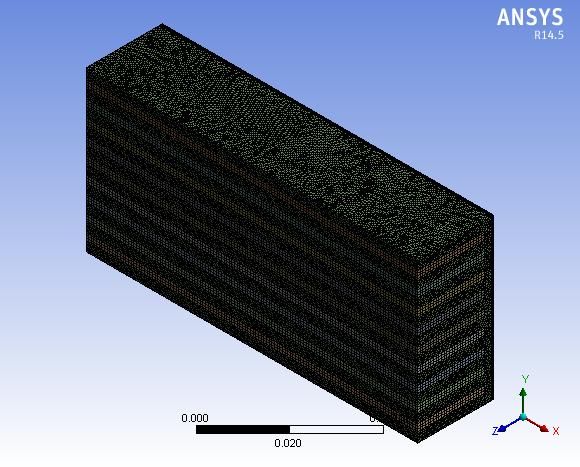
International Conference on Engineering for Sustainable World                                IOP Publishing
Journal of Physics: Conference Series             1378 (2019) 022003   doi:10.1088/1742-6596/1378/2/022003

   The fins that make up an integral part of the heat sink are defined as extended surfaces that use
   conduction-convection effects to enhance heat transfer between the heat sink and the adjoining
   fluid. In the design and optimization of heat sink parameters, it should however be noted that
   the parameters are kind of interdependent on each other [1].

   Due to thermal energy generated arising from the switches operation, proper thermal
   management must be put in place to safe guard the switches, the switches commonly used are
   IRF 3205 MOSFET chips [4]. Thermal energy generated during the switches operation leads to
   increase in temperature of the IRF 3205 MOSFET chips which will ultimately affect its
   performance and can lead to thermally induced failure [5]. The heat sink can be optimized by
   variations to its geometry and material [6].

   The dissipated heat from the switches in the power inverter is transferred to the heat sink through
   case and gap materials. Subsequently this heat is transferred from the heat sink to the ambient
   air. Hence there is need to optimized the heat sink geometry so that estimated junction
   temperature of switch is not greater than the prescribed junction temperature [7], [8].

   Thus a general mathematical optimization of air cool heat sink was derived; the results were
   verified through numerical simulations and experiments. The heat sink optimization is
   performed on the basis of the heat sink geometry [9].

   2.    Mathematical Model of Thermal Dissipation and Heat Sink

   The IRF 3205 MOSFET switches attached to the heat sink have junction temperature which is
   critical to its performance. The dissipated heat from the switches is transferred to the heat sink
   through the case and gap materials. Subsequently this heat is transferred from the heat sink to
   ambient air. It is the ultimate aim to design heat sink geometry so that estimated junction
   temperature of the switches is not greater than the prescribed junction temperature. The
   dissipated power forms an input to the thermal model of the heat sink.

   2.1 Power Dissipation during Switch Operation and Conduction
   Figure 2 shows the electrical to thermal transformation of the IRF 3205 MOSFET switch. The
   capacitor shown model the transient thermal response of the circuit which follows a resistance
   capacitance time constant.

                                                      2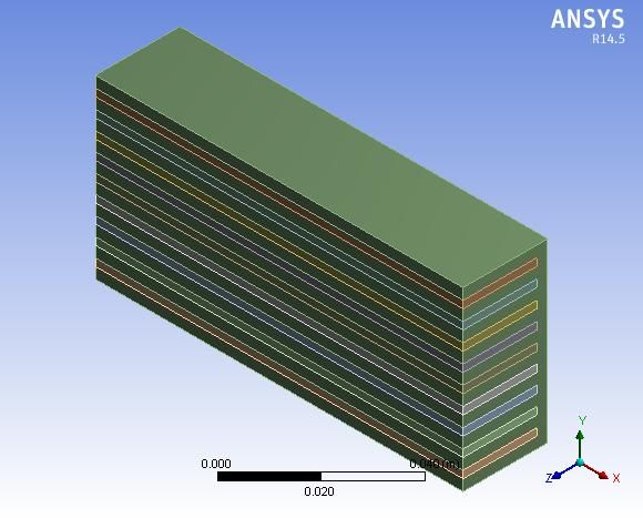
International Conference on Engineering for Sustainable World                                       IOP Publishing
Journal of Physics: Conference Series             1378 (2019) 022003          doi:10.1088/1742-6596/1378/2/022003

                                Figure 2: Principle of Electro – Thermal Analogy

   Temperature becomes an important factor when designing power inverter. Switching and
   conduction losses heat up the silicon of the IRF 3205 switch above its maximum junction
   temperature that causes performance failure, breakdown and worst case fire.

   The total dissipated power in the switches is the sum of the conduction and switching losses
   [10], [11]. When the IRF 3205 MOSFET chip is turned on, the energy losses (E) can be
   calculated as [12], [13]:

                                 E = U × I ×        + Q × U                   (1)

   Where t  is the current rise time, t  is the voltage fall time, I is the drain current, U is
   the Inverter supply voltage (DC), Qrr is the reverse recovery charge. The voltage fall time can
   be calculated as a median of the fall times defined through the gate current as [14]:

                                                t  =                                                      (2)
   Where

                                        t  = (U  R  . i )                                    (3)


                                        t  = (U  R  . i )                                        (4)

                                                        !"#$"
                                             I =        %
                                                                                                            (5)

   where C is the gate-drain capacitance 1, C is the gate-drain capacitance 2, R  is the gate
   Resistance, U is the output voltage from driver circuit, U'*,-, is the plateau voltage.

   The turn off energy losses is expressed as:

                                        E = U × I ×                                               (6)

                                                      3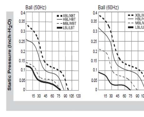
International Conference on Engineering for Sustainable World                                   IOP Publishing
Journal of Physics: Conference Series             1378 (2019) 022003      doi:10.1088/1742-6596/1378/2/022003

   Where t  is the voltage rise time, t  is the current fall time. The voltage rise time can similarly
   be calculated as a median of the rise times defined through the gate current as:

                                              tru =                                                     (7)
   Where

                                      tru1 = (U  R  . I )                                   (8)


                                      tru2 = (U  R  . I )                                      (9)

                                                             !"#$"
                                              I =                                                  (10)
                                                              %

   The total losses due to switching in the chips are function of switching frequency and can be
   obtained as [15]:

                                              P/0 = (E + E )f/0                                 (11)
   All silicon devices provide resistance to the flow of electric current that originates from the
   resistivity of the bulk semiconductor materials. When the device is operating in the ON state
   and the OFF state leakage current, the losses due to conduction in the chips is computed using
   the drain-source ON state resistance (34567 ) [12], [6]:

                                               U (i ) = R  (i ) × i                            (12)
   Where U is the drain source voltage, i is the drain current.
   Therefore, the instantaneous value of the IRF 3205 MOSFET conduction loss is [12]:

                                     P (t) = U (t) × i (t) = R  × i (t)                        (13)
   The total power dissipation due to switching ON and OFF and conduction of the chips is then
   obtained as:
                         P8 = P + P/0 = R  × I 9/ + (E + E )f/0           (14)
   The ON state resistance of the chip is highly temperature dependent, and it can be linearly
   obtained as:
                          R  = R ': × ;1 + 0.005 × ?T@9,A  T': BD           (15)
   Where T@9,A is the operating junction temperature, R ': is the ON state resistance value
   at T': , T': is normally 25oC. The power dissipation varies with the duty ratio and equation
   (14) is re-written as:
                           P8 = Ft  f/0 (R  × I 9/ + (E + E )f/0 )              (16)
   From equation (1) and equation (6), the power dissipated is obtained as:

   P8 = (Ft  f/0 ) G(R  × I   9/ )   + HU × I ×                    + Q × U + U ×

   I ×                 J f/0 K                                                                      (17)

                                                        4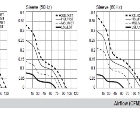
International Conference on Engineering for Sustainable World                                 IOP Publishing
Journal of Physics: Conference Series             1378 (2019) 022003    doi:10.1088/1742-6596/1378/2/022003

   2.2 Thermal Resistance of Heat Sink

   In order to determine the effectiveness of heat sink, a thermal performance metrics has to be
   introduced that take into account the overall heat dissipation, cost function as a weight of heat
   sink and the heat sink geometry of fin spacing, fin length, fin thickness, base thickness and
   number of fins. Figure 3 depicts a diagram of a straight fin heat sink.

                            Figure 3: Heat Sink Thermal Resistance Network [16]

   The hydraulic diameter, dL , of the heat sink channel is defined [17]:
                                                       MN
                                                  dL = O                                              (18)

   And the area, A, perpendicular to flow is expressed as:
                                              A = (n  1)s V L                              (19)
   The wetted perimeter, P, of the duct is obtained as:
                                            P = 2(n  1)(s + L )                            (20)
   From equation (19) and equation (20), the hydraulic diameter of the fluid channel as a function
   of the fin spacing and fin height is then:
                                                        /X
                                                 dL = / X                                    (21)

   For the given fin geometry, the total air flow through the channels creates a pressure drop along
   the heat sink length, L, For laminar flow as [18]:
                                                         Y X
                                              FPX = 1.5 (/Z X )8 VZ                                 (22)
                                                                 [

   Where ] is the density of air kg/m3, ^ is the kinematic viscosity of air m2/s, _Z is volume flow
   rate m3/s. The 1.5 correction factor takes into account the non quadratic channel shape
   characterized by s ` L , where Lf is the fin length.

                                                      5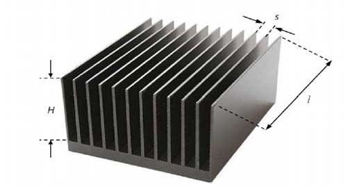
International Conference on Engineering for Sustainable World IOP Publishing
Journal of Physics: Conference Series 1378 (2019) 022003 doi:10.1088/1742-6596/1378/2/022003
For turbulent flow, the drop in pressure is as defined [18]:
bZ ce hZ
X g j
bZ e
?bZ e B
FPa = (23)
hZ
gk.lm *g j .oMj
?bZ ce B
For appropriate fan selection the air flow static pressure characteristic curve is used as shown
in figure 4.
Figure 4: Air Flow and Static Pressure Characteristics [19]
The air flow static pressure characteristic curves are found in the technical data of the fan
manufacturer catalog. The Reynolds number, Re, as a function of the heat sink geometry as
follows [18]:
8
Re = [ (24)
Where u is the velocity of flow, m/s, is the dynamic viscosity, kg/ms. Now
= (25)
qZ
u=N (26)
Where VZ is the volume flow rate, m3/s and A is the cross sectional area, m2. For the heat sink,
the area of flow is obtained as:
A = sL (n 1) (27)
Where n is the number of fins. Substituting equation 25, equation 26, equation 27 and equation
21 into equation 24, gives the Reynold number as:
qZ
Re = ( )(/Z X )
(28)
The Reynold’s number, Re, determine whether the flow is laminar or turbulent. For laminar
flow Re is < 2300 and the Nusselt number, Nu, is defined as [18]:
6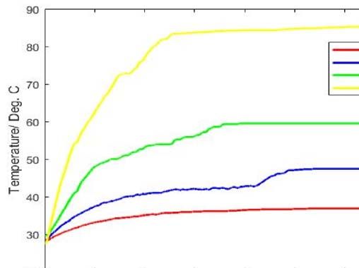
International Conference on Engineering for Sustainable World IOP Publishing
Journal of Physics: Conference Series 1378 (2019) 022003 doi:10.1088/1742-6596/1378/2/022003
{ |.|}~~
Y.owl;,L? . oMxzy .lxzy BD ,L x
NuX = ,L? .MY ' z xz B
(29)
With
X
X=8 (30)
[ %-'
Pr = (31)
For turbulent flow Re > 2300 and the Nusselt number, Nu, is expressed as [18]:
{
;(k.lm * %- .oM) D (%- kkk)'
Nua = zy (32)
.l [(k.lm * %- .oM) ]{ ?' zy B H [ J
e
Properties of air are obtained at mean film temperature, Tf, defined by [20], [21]:
a a
T = (33)
The heat transfer coefficient is thus expressed as:
h = 8[
(34)
From the geometry of figure 1, the thermal resistance of the heat sink is readily expressed as:
e e
[ " e [ " e 8
"! "!
R ,L/ = + (38)
e N
g j
[b
[ " e"!
The governing equations in 2-D solved by the ANSYS Fluent code are defined by the continuity
equation defined by equation (39), momentum equation defined by equation (40) and energy
equation defined by equation (41).
+ = 0 (39)
2 ¢ ¢2
¡
+ £
= £2
(40)
¤ ¢¤ 2 ¤
¡
+ £ = ¥ £2 (41)
Where
¦
¥ = §¨ (42)
©
7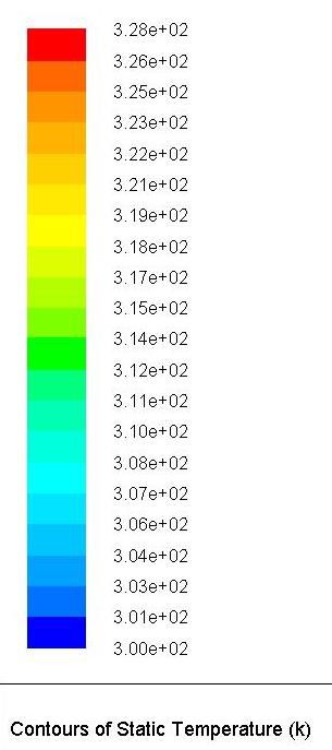
International Conference on Engineering for Sustainable World                                IOP Publishing
Journal of Physics: Conference Series             1378 (2019) 022003   doi:10.1088/1742-6596/1378/2/022003

   3.    Methodology

   The power dissipation of the IRF 3205 MOSFET was derived and fed as input to the generated
   heat sink model. The heat sink was optimized using MATLAB optimization tool, FMINCON,
   to obtained the optimal parameters of the heat sink. The optimized heat sink parameters are;
   heat sink length equal to 0.048m, base thickness equal to 0.0030m, fin length equal to 0.020m,
   fin width equal to 0.1m, fin spacing equal to 0.002m, fin thickness equal to 0.0030m and number
   of fins equal to 10. The thermal performance of the heat sink was done using ANSYS
   computational fluid dynamics. A test rig consisting of a 2.5 K.V. A, 12 VDC power inverter
   was assembled and experimental testing of the optimized heat sink was demonstrated at
   different load conditions. Figure 5 shows the experimental setup.

                                             Figure 5: Experimental Test Rig

   Temperature data were recorded with a K-type thermocouple and a three channel temperature
   logger, MTM-380SD, with real time data logger.

   Figure 6 shows geometric model of the optimized heat sink using Design Modeler in ANSYS
   15.0 Work Bench. While Figure 7 shows the Grid Refinement test image. The dimensions of
   the model are; heat sink length equals 0.048m, base thickness equals 0.003m, fin height equals
   0.02m, heat sink width equals 0.1m, fins spacing equals 0.003m, fin thickness equals 0.003m
   and number of fins equals 10.

   The flow is assumed to be steady, laminar and incompressible. The cooling fluid is air with
   constant thermo-physical properties. Heat transfer within the geometry is a combination of
   conduction and convection heat transfer. The mesh was generated automatically by the ANSYS
   mesh tool while the orthogonal quality and skewness were monitored to give better mesh quality
   than the expected limits. Grid refinement tests were carried out and results of maximum
   temperature on the heat sink base converged when the number of elements was 914,534. The
   governing equations in 2-D solved by the ANSYS Fluent code with their boundary conditions
   are defined by the continuity equation defined by equation (39), momentum equation defined
   by equation (40) and energy equation defined by equation (41).

                                                      8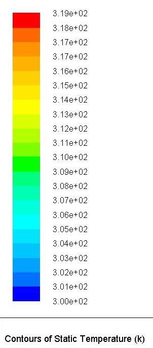
International Conference on Engineering for Sustainable World IOP Publishing
Journal of Physics: Conference Series 1378 (2019) 022003 doi:10.1088/1742-6596/1378/2/022003
+ = 0 (39)
2 ¢ ¢2
¡
+ £
= £2
(40)
¤ ¢¤ 2 ¤
¡
+ £ = ¥ £2 (41)
Where
¦
¥ = §¨ (42)
©
The cooling fluid is air with an inlet temperature of 27oC, symmetry boundary conditions are
specified.
Figure 7: Grid refinement image
Figure 6: Modelled Heat sink
Geometry
4. Results and Discussion
4.1 Simulation Results using ANSYS FLUENT Computational Fluid Dynamics Software
Simulations results produced by ANSYS FLUENT solver are presented to determine the
performance of the heat sink at different load conditions. The ANSYS model employed a dense
mesh containing 12000 nodes, 234 temperature monitoring points and 56 time steps to ensure
accurate results. The inputs to the solver are the dissipated power, air flow velocity, ambient
temperature and pressure drop termed the boundary conditions.
9International Conference on Engineering for Sustainable World IOP Publishing
Journal of Physics: Conference Series 1378 (2019) 022003 doi:10.1088/1742-6596/1378/2/022003
4.1.1 Numerical Result at a Pulse Load of 300 W
Figure 8 shows the temperature contour plot as obtained from the simulation result of the
optimized heat sink at pulse load of 300 W.
Figure 8: Temperature contour plot at 300W Pulse Load from ANSYS simulation
The thermograph represents the temperature distribution across the surface of the heat sink, it
can be seen that the hottest point is at the heat sink base and has a maximum temperature of
307 K.
4.1.2 Numerical Result at a Pulse Load of 460 W
Figure 9 shows the temperature contour plot as obtained from the simulation result of the
optimized heat sink at pulse load of 460W in ANSYS.
The thermograph represents the temperature distribution across the surface of the heat sink, also
it can be seen that the hottest point is at the heat sink base and has a maximum temperature of
319 K which is an increase of 3.9% when compared to the pulse load of 300 W.
10International Conference on Engineering for Sustainable World IOP Publishing
Journal of Physics: Conference Series 1378 (2019) 022003 doi:10.1088/1742-6596/1378/2/022003
Figure 9: Temperature contour plot at 460 W Pulse Load from ANSYS simulation
4.1.3 Numerical Result at a Pulse Load of 600 W
Figure 10 shows the temperature contour plot as obtained from the simulation result of the
optimized heat sink at pulse load of 600 W.
Figure 10: Temperature contour plot at 600 W Pulse Load from ANSYS simulation
11International Conference on Engineering for Sustainable World IOP Publishing
Journal of Physics: Conference Series 1378 (2019) 022003 doi:10.1088/1742-6596/1378/2/022003
The thermograph represents the temperature distribution across the surface of the heat sink,
again it can be seen that the hottest point is at the heat sink base and has a maximum temperature
of 328 K which is a further increase of 2.8% when compared to the pulse load of 460 W.
4.1.4 Numerical Result at a Pulse Load of 1015 W
Figure 11 shows the temperature contour plot as obtained from the simulation result of the
optimized heat sink at pulse load of 1015 W.
The thermograph represents the temperature distribution across the surface of the heat sink,
clearly it can be seen that the hottest point is at the heat sink base and has a maximum
temperature of 357 K which is 8.1% increase when compared to the pulse load of 600 W.
Figure 11: Temperature contour plot at 1015 W Pulse Load from ANSYS simulation
From the results of the numerical simulation, as the pulse load increases, the maximum
temperature at the base of the heat sink increases. This is as expected as the dissipated power
increases with pulse load due to the increase in the drain current in the IRF 3205 MOSFET, for
all load conditions the maximum junction temperature of the switches are not exceeded.
4.2 Comparison between Experimental and Numerical Results
The experimental data plots were compared to the numerical results obtained using the ANSYS
FLUENT solver. Figure 12 shows the experimental data plots of temperature against time at
various inverter load conditions of 300 W, 460 W, 600W and1015 W respectively. The MTM-
380SD used for temperature data collection has a resolution of 0.1oC and an accuracy of ± 0.5%
+ 0.5oC.
12International Conference on Engineering for Sustainable World IOP Publishing
Journal of Physics: Conference Series 1378 (2019) 022003 doi:10.1088/1742-6596/1378/2/022003
Figure 12: Temperature -Time graphs at various Inverter Loads
In Table 1, a summary of results obtained numerically and from experiments are presented and
from the tables one can see the percentage increase in temperature as the pulse loads increases.
Results obtained show that the percentage deviation between the ANSYS simulation and
experimental temperature for a pulse load of 300W is 8%, for a pulse load of 460W is 3%, for
a pulse load of 600W is 8%, for a pulse load of 1015W is 2% as shown in Table 2. Thus the
experimental data closely validates the simulated results. Table 2 also presents the relative error
between the numerical and experimental results calculated relative to the ambient temperature.
In all test cases of pulse loads, the maximum junction temperature of the IRF 3205 MOSFET
switch is not exceeded and the power inverter can thus be safely and reliably operated. This
shows that the optimised heat sink was able to contain the heat generated during the switching
and conduction cycle of operation of the switches.
Table 1: Comparison between temperature increase for different pulse loads
Numerical results Experimental results
Steady-State Temp % Steady-State %
S/N Load /W (oC) Increase in Temp. Temp ( oC) Increase in Temp.
1 300 34 36.9
2 460 46 35.3 47.4 28.5
3 600 55 19.6 59.7 25.9
4 1015 84 52.7 85.4 43
13International Conference on Engineering for Sustainable World IOP Publishing
Journal of Physics: Conference Series 1378 (2019) 022003 doi:10.1088/1742-6596/1378/2/022003
Table 2: Percentage difference in results obtained numerically and experimentally
S/N Load Numerical Experimental % Relative
(W) Steady-state temp. ( C)
o
Steady state temp. Deviation error (%)
(oC)
1 300 34 36.9 8 34
2 460 46 47.4 3 7
3 600 55 59.7 8 15
4 1015 84 85.4 2 2
5. Conclusion
Power inverters are essentially for supplying energy for today’s society in a more efficient,
sustainable and controllable manner. Thermally induced failure modes are the main cause of
power inverter reliability issues. With the aim of efficiently dissipating the heat generated from
the power inverter, a heat sink model was then developed and optimized using the MATLAB
FMINCON optimization tool. The resulting optimized heat sink variables are; fin spacing equal
to 0.005m, fin height equal to 0.02m, number of fins equal to 10, fin thickness equal to 0.003m,
heat sink length equal to 0.1m, heat sink base thickness equal to 0.004m, from which width of
the heat sink equal to 0.075m, fin spacing ratio of 0.6667. The static pressure of the fan is
obtained as 21.7113N/m2 and from the fan characteristic curve; the volume flow rate of air is
0.03065m3/s and the selected fan model is 2123HSL with dimensions 120mm square by 38mm.
Thermal performance of the optimised heat is carried out using ANSYS Computational Fluid
Dynamics (CFD) software. The maximum simulated and experimented recorded temperatures
are 84oC and 85.4oC. The results obtained from simulations and experimental data are in good
correlation with a maximum of 8 percent deviation at a load of 600W.
References
[1] Barker C. R., Olson R. E., Lindquist S. E., Cease D. A., Sobolewski R. S. (1997). High
Performance Fan Heat Sink Assembly, US patent, issue 19, patent number 5597034.
[2] Lee S. (1999). Optimum Design and Selection of Heat Sinks. Aavid Engineering Inc.
Laconia, New Hampshire
[3] Mostafavi G. (2010). Natural Convective Heat Transfer from Interrupted Rectangular
Fins University of Tehran.
[4] Shinohara S. (2002). Analysis of power losses in MOSFEt Synchronous Rectifiers by
using their design parameters. Proceedings of the 10th international symposium on power
semiconductor devices and IC’s .ISPSD’98 (IEEE).
[5] Schlapbach U., Rahimo M., Von Arx C., Mukhitdinov A. (2007). 1200V IGBTs
Operating at 200oC? An investigation on the potentials and the design constraints in the
19th International Symposium on Power Semiconductor Devices and ICs (ISPSD), Jeju,
South Korea, pp. 9 – 12.
[6] Drofenik U. Laimer G., Kolar J. W. Theoretical Converter Power Density Limits for
Forced Convection Cooling Power. Electronics Systems Laboratory, ETH Zurich.
[7] Majumdar G. (2007). Recent Technologies and Trends of Power Devices in the 14th
International Workshop on Physics of Semiconductor Devices (IWPSD), Mumbai, India,
pp. 1 – 6.
[8] Franquelo L. G., Leon J., Dominguez E. (2009). New Trends and Topologies for High
Power Industrial Applications: the multilevel Converters solution in the International
14International Conference on Engineering for Sustainable World IOP Publishing
Journal of Physics: Conference Series 1378 (2019) 022003 doi:10.1088/1742-6596/1378/2/022003
Conference on Power Engineering, Energy and Electrical Drives (POW-ERENG),
Lisbon, Portugal, pp. 1-6.
[9] Shin D. Thermal Design and Evaluation Methods for Heat Sink. E-CIM Team, Corporate
Technical Operations, Samsung Electronics Co.
[10] Rajapakse A. D., Gole A. M., Wilson P. L. (2005). Approximate Loss Formulae for
Estimation of IGBT Switching Losses through EMTP-Type Simulations Presented at the
International Conference on Power Systems Transients (IPST 05) in Montreal, Canada,
Paper No. IPST05-184.
[11] Haaf P., Harper J. (2007). Understanding Diode Reverse Recovery and its effect on
Switching Losses Fairchild Power Seminar A25-A28.
[12] Graovac D., Pürschel M., Kiep A., (2006). MOSFET Power Losses Calculation using the
Data-sheet parameters. Application Note, V I.I, Infineon Technologies Austria AG, pp
2-6.
[13] Jauregul D., Wang B., Chen R. (2011). Power Loss Calculation with common Source
Inductance consideration for synchronous Buck Converters. Application Report, Texas
Instruments.
[14] Keagy M. (2002). Calculate Dissipation for MOSFETs in High Power Supplies.
Electronic Design.
[15] Blinov A., Jalakas V. D. (2011). Loss Calculation Methods of Half-Bridge Square-Wave
Inverters Electronics and Electrical Engineering, Estonia, ISSN 1392-1215, pp. 9-11.
[16] Onoroh F., Enibe S. O., Okolie P. C. (2015). Optimisation Techniques for Thermal
Management in an IRF 3205 Mosfet Switches. Journal of Emerging Trends in
Engineering and Applied Sciences (JETEAS) 6(6) 399-404.
[17] Kays W.M. and Crawford M.E. (1993). Convective heat and mass transfer. 3rd edition
McGraw-Hill book companies.
[18] Baehr H. D., Stephen K., (1998). Heat and Mass Transfer. 3rd Edition. ISBN 3-540-
64458-X, Springer, pp. 220-221, 259-262, 350-355.
[19] Sunon (2002). AC Axial Fan and Blower. http://www.sunon.com. [Retrieve 9th
November 2014].
[20] Rogers G., Mayhew Y., (1992) Engineering Thermodynamics Work and Heat Transfer.
4th edition, Delhi: Pearson Education. pp. 509-518.
[21] Eastop T.D., McConkey A. (1993). Applied Thermodynamics for Engineering
Technologies. 5th edition. Delhi: Pearson Education, pp. 577-583.
15You can also read