Where's Wally Now? Deep Generative and Discriminative Embeddings for Novelty Detection
←
→
Page content transcription
If your browser does not render page correctly, please read the page content below
Where’s Wally Now?
        Deep Generative and Discriminative Embeddings for Novelty Detection

                                Philippe Burlina, Neil Joshi, and I-Jeng Wang
                            Johns Hopkins University Applied Physics Laboratory
                         {philippe.burlina, neil.joshi,i-jeng.wang}@jhuapl.edu

                          Abstract                                     learning abilities, where the ability to perform novelty de-
                                                                       tection allows a robot to trigger human-machine dialogue
   We develop a framework for novelty detection (ND)                   to seek information on novel objects it encounters; (2) per-
methods relying on deep embeddings, either discriminative              forming medical diagnostics for rare diseases (e.g., my-
or generative, and also propose a novel framework for as-              opathies) – for which prior observations are sparse or un-
sessing their performance. While much progress was made                available – and using novelty detection to pre-screen pa-
recently in these approaches, it has been accompanied by               tients and refer them to clinicians; and (3), zero-shot se-
certain limitations: most methods were tested on relatively            mantic learning leveraging novelty detection to improve
simple problems (low resolution images / small number of               zero-shot classification performance by turning a general-
classes) or involved non-public data; comparative perfor-              ized / uninformed zero-shot problem into an easier informed
mance has often proven inconclusive because of lacking                 problem (where it is known if the object comes or not
statistical significance; and evaluation has generally been            from a novel class) for which higher performance can be
done on non-canonical problem sets of differing complexity,            achieved [29, 38].
making apples-to-apples comparative performance evalua-                   Prior work Past work in ND goes far and wide, and
tion difficult. This has led to a relative confusing state of af-      started with methods primarily grounded on classical ma-
fairs. We address these challenges via the following contri-           chine learning (for recent surveys see [14, 31, 33], and more
butions: We make a proposal for a novel framework to mea-              domain specific surveys [2, 4, 25]), including approaches
sure the performance of novelty detection methods using a              such as [7,13,15]. For instance, [7] used image features and
trade-space demonstrating performance (measured by RO-                 Support Vector Data Description (SVDD) for ND applied to
CAUC) as a function of problem complexity. We also make                hyperspectral imaging. [13] used convolutional sparse mod-
several proposals to formally characterize problem com-                els to characterize novelty. Novel multiscale density estima-
plexity. We conduct experiments with problems of higher                tors working for high dimensional data were developed and
complexity (higher image resolution / number of classes).              applied to ND in dynamic data in [15]. By contrast, repre-
To this end we design several canonical datasets built from            sentation learning via deep learning (DL) has offered novel
CIFAR-10 and ImageNet (IN-125) which we make available                 ways to implement ND [18, 25, 36], with methods falling
to perform future benchmarks for novelty detection as well             into two main categories: generative and discriminative.
as other related tasks including semantic zero/adaptive shot              Recent ND via DL Novelty detection using discrimina-
and unsupervised learning. Finally, we demonstrate, as one             tive deep learning approaches were developed first based
of the methods in our ND framework, a generative novelty               on deep embeddings computed by processing the image
detection method whose performance exceeds that of all re-             through deep discriminative networks, including deep con-
cent best-in-class generative ND methods.                              volutional neural nets (DCNNs), deep belief networks
                                                                       (DBNs), or recursive neural nets (RNNs). In [18] discrimi-
                                                                       native embeddings via DBNs and DCNNs were used along
1. Motivation, prior work, and contributions                           with one class SVM (1CSVM) to detect novelty. Most
                                                                       recently, generative approaches, principally via generative
   Motivation Novelty detection (ND) methods [7, 13–                   adversarial networks (GANs) or variational autoencoders
15, 18, 31, 33, 36, 38] have applications in a wide array of           (VAEs) have been embraced for representation learning for
use cases including in semi/unsupervised learning, lifelong            novelty detection [1, 3, 8, 16, 20, 21, 24, 26, 28, 32, 36, 41].
learning and zero-shot learning [29]. Application examples             Most approaches focus on GANs’ ability to offer varied
include: (1) robotic applications with lifelong and open set           means for embedding (e.g., in latent space, using the en-

                                                                    111507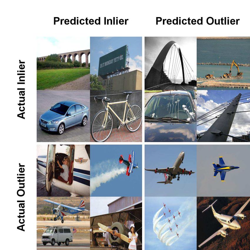
Figure 1. ND framework We propose a novelty detection (ND) framework along with a principled approach for evaluating ND methods
which computes performance as (ROCAUC)=f(problem complexity). Our ND framework performs novelty detection in two main steps,
by a) embedding the image either via generative or discriminative networks, then b) computing a novelty score. Specifically: the left
block shows our use of two types of discriminative embeddings (here via VGG16) using either GAP features XGAP 512 computed from the
output of the convolutional layers (marked as ConvNet) or the concatenation of all features from the ConvNet layers as well as the fully
connected layers (marked as MLP), producing an embedding vector denoted as XM U LT I . An alternative in our framework consists of
using a generative embedding: using the latent space vector of a GAN (here we use Ganomaly [3]), denoted as XGAN . Embedded feature
vectors are then used to compute a novelty score via one of several approaches: either one class SVM (1CSVM), local outlier factor (LOF),
elliptic envelope (EE) or isolation forest (IF). The Ganomaly architecture uses as a discriminator a series of encoder (DE1 ) decoder (DD )
and encoder (DE2 ). In our framework we directly leverage the latent vector XGAN output of DE1 as embedding for ND.

                 Discriminative embedding                                             Generative embedding

                                                                                                 G        DE1   DD   DE2
                                                                 Input image

                          ConvNet MLP
                                                                concatenate                                          D
                                                                        XMULTI
                                                     XGAP512
                                                                    either
                                                                                          XGAN
                                                                 Novelty score
                                                               (LOF, OCSVM, EE,            Novelty 0/1?
                                                                      or IF

coder or decoder network for embeddings, or using the dis-                   making apples-to-apples comparisons due to the lack of re-
criminator’s output, or other more complex ways) where                       peated testing protocols. For instance, even when the same
novelty scores can then be computed. Looking at the core                     dataset is used, say MNIST, choosing different schemes for
contributions: AnoGAN in [36] used DCGAN [34], and                           partitioning inlier and outlier classes results in large differ-
compared several GAN embedding and novelty measure                           ences in difficulty for the resulting novelty detection prob-
approaches that included inverting the mapping from im-                      lems. Quantitatively measuring ND problem complexity
age to latent space, and measuring reconstruction error. It                  has never before been addressed, and is itself a complex
demonstrated improvements in area under the curve (AUC)                      challenge. Finally, most past studies have used rather sim-
when compared to simply using the GAN discriminator                          ple problems with small number of classes and low resolu-
for novelty detection. It did so in experiments perform-                     tion images, making it hard to predict how these methods
ing pixel-based anomaly detection on OCT images, using                       would generalize in more complex, in-the-wild situations.
49 OCT images and 64 × 64 sliding windows for pixel                              Contributions of this work
ND. A related method, ADGAN, was applied to whole im-                            We address ND, defined as the problem of training on
age anomaly detection [16] and tested on images includ-                      inlier data not corrupted by outliers, and making inferences
ing MNIST (28 × 28 images) and CIFAR-10 (32 × 32)),                          on new observations to detect outliers. To address the ND
showing some improvement over past GAN-based meth-                           challenge we make the following contributions: using a
ods. [41] proposed a related approach using a more effi-                     simple taxonomy of methods, we develop a framework for
cient GAN implementation and a modified loss function,                       ND methods including both discriminative and generative
and tested it on network intrusion data and a simple image                   embeddings, coupled with various approaches for measur-
dataset. Recently, [3] developed an approach using GANs                      ing novelty. We make a proposal for a principled method
where the discriminator network structure was composed                       for evaluating the performance trade space of ND methods,
of an encoder/decoder/encoder path, providing two latent                     that expresses computed performance (AUC) as a function
embedded spaces, and the novelty score was measured via                      of measured problem complexity. We propose and discuss
the reconstruction error between two latent spaces. This re-                 several methods for quantitatively assessing problem com-
sulted in best in class performance when compared to all                     plexity based on semantic, information theoretic, and Bayes
aforementioned methods on CIFAR-10 and MNIST.                                error based approaches. We propose, release, and test on
   Challenges Given the explosion of methods relying on                      canonical datasets and protocols for ND assessment, based
deep embeddings for ND, one would hope to bring some or-                     on CIFAR-10 and ImageNet with higher image resolution
der and address challenges in interpreting what constitutes                  and number of classes. Finally, we demonstrate that one
actual progress in performance and what led to performance                   of our ND generative methods exceeds performance when
improvement. Some challenges stem from the difficulty in                     compared to all prior generative methods reported thus far.

                                                                      121508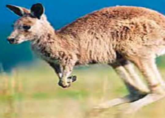
2. Methods                                                          classes truly are unseen by the model. To take a stronger
                                                                    stand we also pose the same restrictions on inlier classes.
   We describe next the main approaches used herein in
our ND framework using generative or discriminative deep
embeddings. The family of algorithms we consider uses               Generative embeddings Generative adversarial net-
the following pipeline: a) computation of deep embedding,           works (GANs) are a deep generative approach which learns
via discriminative methods, or using GANs for generative            to generate novel images from a training dataset. GANs
methods (Section 2.1) leading to an embedded vector X of            are composed of two networks that work with adversar-
an input image I; b) PCA dimensionality reduction and nor-          ial losses. One network performs image generation, using
malization of X, and then followed by c) measuring novelty          for example up-convolutions, that map a randomly sampled
scores (Section 2.2). As novelty detection is trained on a set      vector from latent space to image space, thereby generat-
of inlier classes only, and testing is carried out on a set of      ing synthetic images. Synthetic images thus created are
images from inliers and outlier (yet unseen) classes, step (c)      then fed to a discriminative network (along with real im-
broadly consists of using training exemplars to character-          ages), and this network is trained to classify generated vs
ize some notion of “distance” computed from a test image            real images. The discriminative network may use a cross-
to training inlier exemplars, which is then translated into a       entropy loss function or Jensen-Shannon divergence which
novelty score. This framework and its various subcompo-             it minimizes, while the generative network – tries to fool the
nents are illustrated in Figure 1.                                  discriminative network, and to maximize this loss function.
                                                                    At convergence, the discriminator has learned to discrimi-
2.1. Discriminative and generative embeddings for                   nate between real and fake images, while the generator has
      ND                                                            leaned to generate realistic looking images that are essen-
Discriminative embeddings In this work we start by                  tially sampled from the original training image distribution.
computing deep embedding on the image using a pre-                      One possibility for a GAN embedding used for novelty
trained DCNN, here using VGG-16 [35, 37]. The structure             detection consists of using the latent space. Computing it
of VGG-16 is recalled here only for convenience: it is first        could be done by a network that performs an inversion of
composed of a series of convolutional blocks:                       the generative mapping (an encoder network) that takes an
                                                                    image as input and generates a latent vector as output. As an
 1         2          3          4          5
C(2,64) → C(2,128) → C(3,256) → C(3,512) → C(3,512) →F              alternative method, this latent vector can be fed back again
                         i
                                                                    through the GAN’s generator network, in essence creating
where a block named C(n    l ,nd )
                                   denotes the ith block com-       a reconstruction of the original input image. One can then
posed of nl successive convolutional layers of size 3 × 3           send this reconstruction through the GAN’s discriminator
with depth nd , each of which is followed by rectified linear       network to perform novelty detection.
units (ReLU) activation, and where each such block is fol-              An alternate method to obtain the latent vector is via the
lowed by a pooling layer. This is then followed by flattening       method in [3] which relied on a discriminator that used a de-
F and then fed to three successive fully connected layers on        coder/encoder/decoder structure. Because of this structure,
a vector of width 4096:                                             by training the discriminator, one essentially obtains an en-
                 1
              F C4096      2
                      → F C4096      3
                                → F C4096                           coder that yields a latent space mapping “for free” (with-
                                                                    out inversion needed). Unlike [3], we use this approach in
Our embeddings consist of computing both GAP (global av-            our framework as a means of producing a generative latent
erage pooling) features , denoted XGAP 512 , and multi-layer        space embedding for novelty detection. We call this vector
(XM U LT I ) features. The GAP features are computed out of         embedding XGAN . In our approach, we use XGAN via the
                 5                                                  ND scoring methods described in the next section.
the output of C(3,512)   and we apply the average operator to
each of the 512 feature planes resulting in a 512-long fea-             Finally, we compare our ND generative approach to three
ture vector. XGAP 512 feature embedding forms a represen-           methods: 1) the original Ganomaly ND scheme in [3],
tation of input images that can be interpreted to contain low       which relies on computing the latent vector reconstruction
and mid level semantic information. In addition we also use         error between the output of the first and second encoder in
as alternate embedding the concatenated feature outputs out         the discriminator (See Figure 1). 2) Alternatively, the image
of all layers (convolutional and fully-connected), denoted          reconstruction error can be used as a score of novelty, as is
as XM U LT I , of total dimension 9664. Feature computation         considered in [36, 41]. [41] in particular employed a nov-
is followed by dimensionality reduction using PCA (with             elty score based on a modification of the AnoGAN in [36].
dimension equal to 120). Since this approach uses a pre-            We use it here also for performance comparisons and de-
trained network, note that in experiments reported later, care      note it as ND-EGAN [41] (for “efficient” GAN). 3) An-
is taken that no class used for pre-training the DCNN in Im-        other principle for GAN-based ND is based on the hypoth-
ageNet is used also as an outlier class to ensure that outlier      esis that the discriminator may be used to detect anomalies.

                                                                 3
                                                                 11509
We use a variation of this method exploiting the discrimi- resulting ND performance, should depend on how close the
nator of Wasserstein GAN (WGAN) [5] which we denote inlier and outlier are in distribution or semantics. Here we
“ND-DGAN’. have different choices for closeness:
One possible approach to complexity is to assess how
2.2. Novelty scores semantically related the outlier classes are to inlier classes.
Novelty detection is done by computing novelty scored This could be achieved by looking at proximity in a hier-
on the aforementioned XGAP 512 , XM U LT I , and XGAN archical class representation (e.g. ImageNet WordNet rep-
embedding vectors. We use four approaches which essen- resentation). However, one challenge with this approach is
tially measure the departure of a test vector X compared to that semantic closeness would depend on the specific hier-
a set of inlier samples, used for training. These are briefly archical representation utilized.
reviewed below (for more details see the appendix): As an alternative, we opt for complexity assessment by
LOF The first approach uses local outlier factor (or characterizing closeness in distribution, here to be solved
“LOF”) [9]. LOF computes a novelty score based on as- by evaluating distances of probability density of embedded
sessing the local density of points around a test point when vectors lying in high dimensional spaces. However, this
compared to the density measured for each of this point’s endeavor is itself still an open research problem. Two ap-
neighbours. Intuitively, if a test point’s density is lesser than proaches could be considered:
its neighbours’ densities, the point may be an outlier. KLCA: KL-divergence based Complexity Assess-
1CSVM The second approach here uses a one class sup- ment A first possibility is to characterize the distance of
port vector machine (or “1CSVM”) [7, 39]. 1CSVM is a distributions (inlier and outlier) via information theoretic
large-margin non-parametric classifier that essentially pro- measures, to characterize ND complexity, e.g. using cross-
ceeds by bounding a set of training inlier exemplars via the entropy, earth moving distance or KL divergence. The com-
smallest enclosing hypersphere. In loose terms (see ap- putation of these measures in general, and KL divergence in
pendix for precise details) the novelty score is then a dis- particular, in high dimensions, is still an open problem for
tance from the test vector to the weighted centroid of the which recently some approaches have been proposed. We
support vectors on this hypersphere. used in particular the method in [40] which leverages effi-
IF Isolation forest (later termed “IF”) is another novelty cient K nearest neighbour (KNN) to compute KL. We call
detection method used here [27]. It is akin to random forests this method KLCA (for KL-based complexity assessment).
in that it consists of building random CART tree structures BERCA: Bayes error rate complexity assessment We
on the training data and exploiting the fact that outliers typ- propose a second approach for characterizing complexity
ically stand isolated in a branch close to the root of the tree. which consists of assessing the complexity metric as the
Random features are selected and splits are computed on Bayes error rate of the two class problem associated with
these features. The path from the root to a feature vector the one class problem partition. We denote this via the
averaged over a set of random trees is taken as isolation acronym “BERCA”. Following this route, we consider the
score and therefore (short meaning isolated) used as nov- two class classification problem Bayes decision rule, i.e. the
elty score. rule that minimizes the probability of error P ∗ . We compute
EE Finally, we also use an ND score that takes the el- the empirical estimate of this error via KNN. Denoting by
liptic envelope (later termed “EE”) obtained by assuming a kknn the numbers of neighbours used in KNN and nknn the
Gaussian distribution fit to the inlier training exemplars. numbers of samples used, we recall [17] that the knn error
In subsequent experiments, for nomenclature: we denote rate P is such that P ∗ ≤ P ≤ P ∗ + ǫ, where ǫ → 0 when
the complete method applying a ND method “XXX” on fea- kknn , nknn → ∞. Henceforth, we use the Bayes error rate
ture type “YY” by “XXX/YY” (e.g., EE applied to GAP512 computed from the empirical KNN error rate estimate as
is denoted “EE/XGAP 512 ”). the problem complexity metric. We use numerical values of
kknn = 10 and nknn = 1000.
2.3. Characterizing ND problem complexity Standardizing the performance evaluation
For comparing the different deep learning novelty detec- Finally, equipped with the complexity measures above,
tion approaches here, we use a set of canonical test prob- we propose that for apples-to-apples comparisons, ND al-
lems mixing inlier and outlier classes: we thereby obtain gorithmic performance be characterized in a trade space
a wide range of problems of varying complexity. We en- that expresses computed performance, measured in terms
deavor to characterize this complexity via some quantita- of ROCAUC, as a function of complexity of the ND prob-
tive measure, to allow for an apples-to-apples comparison lem where this performance was evaluated (i.e. AU C =
of problems of similar complexity. Our final goal is to as- f (complexity)). This is to be displayed as box plots since
sess how well the proposed ND methods perform for differ- the complexity of problems will vary, as will also the result-
ent complexity regimes. Intuitively, the complexity, and the ing performance range for a given complexity bin.
141510Figure 2. Examples of images for one of the problems run in IN- case, we perform experiments on SIMO and MISO prob-
125. In this example 9 inlier classes are randomly selected from
lems defined above for nc = 10 classes. In each problem
the IN-125 dataset (including bikes, bridges, etc..), and one outlier
case, we run 10 experiments, circularly rotating the single
class (airplane) is also selected. We show examples of correct and
incorrect novelty detection. For this experiment AUC=0.896 inlier (SIMO) or single outlier (MISO) every time. We then
evaluate the AUC performance averaged across all 10 ex-
periments (shown in Table 1).
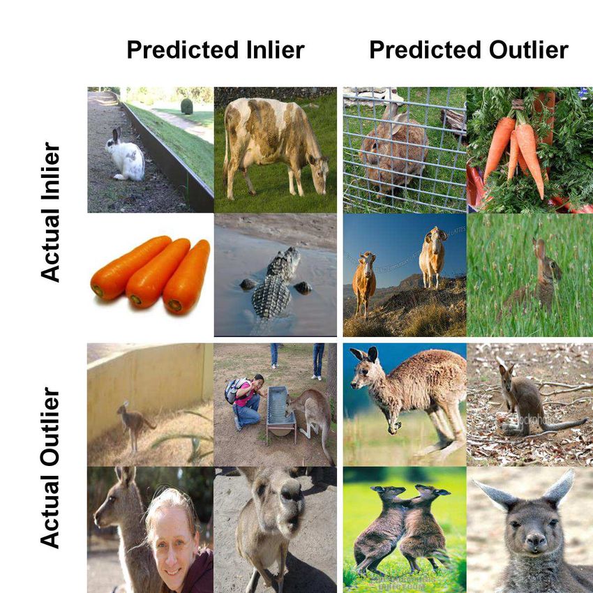
Figure 3. Examples of images for one of the problems run in IN-
125. In this example 9 inlier classes are randomly selected from
the IN-125 dataset (including bunnies, carrots, cows, etc..), and
one outlier class (Kangaroo) is also selected. We show examples
of correct and incorrect novelty detection. Most incorrect classifi-
cations result from confusing factors such as multiple objects and
humans, or bunnies/kangaroo similarity in appearance. For this
experiment AUC=0.878
3. Standardizing ND problem structure and
canonical datasets
We also propose to standardize the data used for evalu-
ating ND around two main datasets with low and high reso-
lution images and two main protocols for choosing inlier vs
outlier class partitioning, described next.
MISO and SIMO problems In general, ND methods
operate on the assumption that they are trained on inliers
only, while testing is carried out on a set of inliers and
outlier-class items, an assumption which is deemed to be
semi-supervised. In addition, partitions of inliers and out- IN-125 Since prior work on ND has consisted mostly of
liers sets can include either single or multiple classes. With testing on simple datasets (MNIST and CIFAR-10), in this
that in mind, we consider two types of problems, and we work, we construct a reference dataset composed of 125 Im-
adopt the following nomenclature: Single (class) Inlier, ageNet classes (termed “IN-125”) on which we additionally
Multiple (class) Outlier problems (termed “SIMO” hence- evaluate the ND methods described above. Note that, by de-
forth), and Multiple (class) Inlier, Single (class) Outlier sign, none of the 125 classes used here in IN-125 belongs
problems (called “MISO”). to the original 1000 ImageNet competition classes that are
Recalling our first use case of an exploring robot as an il- used for training ConvNets like VGG16, so as to avoid
lustrative example, and assuming the existence of nc classes issues that our ND problems may include outlier classes
in the universe, SIMO problems can be thought of as one- that in fact were used for pre-training weights of VGG-16
vs-all problems, in which the robotic agent bootstraps its (or any other network used for discriminative embedding),
knowledge of the universe with a single starter inlier class, which would invalidate the assumptions these classes have
and we perform experiments that evaluates on that same in- not been seen previously.
lier class, plus n − 1 other outlier classes that the agent may IN-125 increases complexity along two challenges when
encounter, while doing exploration. MISO problems can be compared to ND experiments conducted on prior ND stud-
seen as leave-one-out problems, where the ND method is ies in that (a) the images’ resolutions are higher and (b) the
trained on nc − 1 inlier classes, and tested on that same set number of exemplars per class is about one order of magni-
of inlier classes, plus the remaining outlier class. tude lower compared to datasets like CIFAR-10 or MNIST.
CIFAR-10 As a baseline, we evaluate ND methods on We release the specification [11] of this dataset for future
the CIFAR-10 dataset, which contains 10 common classes. comparisons, which consists of the set of problems, each
This dataset has a large number of images per class (6000), of which we detail by providing the list of classes used as
but coarse image resolution (32x32 RGB images). In this inliers and outliers.
5
115114. Experiments and performance characteriza- Figure 4. AUC=f(c) (AUC as a function of problem complexity)
for 125 problems in IN-125 (1CSVM applied to GAP features)
tion
jhu150_LOO_LIMIT_10 - 1CSVM*
0.9
We run experiments on the datasets detailed above. The
results of applying our ND framework to two IN-125 prob- 0.8
lems is exemplified in Figures 2 and 3. We demonstrate the
0.7
use of the performance evaluation framework we designed
whereby we express performance, measured in terms of 0.6
AUC
AUC, as a function of complexity for each of the approaches 0.5
to ND described in this study. We also use the set of se-
lected problems described in the previous section. For each 0.4
problem we show the distribution of AUC=f(complexity). 0.3
0.00 - 0.06 0.06 - 0.10 0.10 - 0.14 0.14 - 0.18 0.18 - 0.21 0.21 - 0.25 0.25 - 0.29 0.29 - 0.32 0.32 - 1.00
We first performed complexity assessment using KLCA. Complexity
Results suggested that it is not an effective empirical com-
plexity measure in that KL divergence did not always cor- Figure 5. AUC=f(c) (AUC as a function of problem complexity)
relate or predict the performance of ND algorithms. This is for 125 problems in IN-125 (Elliptic Envelope applied to GAP
likely due to the issue of attempting to compute KL for dis- features)
tributions that don’t have overlapping support everywhere,
jhu150_LOO_LIMIT_10 - Elliptic Envelope
a problem which is exacerbated by the use of a limited num- 0.9
ber of points in high dimensional spaces.
0.8
We next evaluated performance as a function of BERCA
and plot in Figs 4-7, for GAP512 features, whisker plots 0.7
of the AUC as a function of the BERCA complexity, for 0.6
AUC
each of the main ND scoring methods (1CSVM, LOF,
0.5
IF and EE). The plots demonstrate the effectiveness of
this approach in comparing methods. It can be observed 0.4
that in general performance decreases as BERCA com- 0.3
plexity increases for all methods, with graceful degrada- 0.00 - 0.06 0.06 - 0.10 0.10 - 0.14 0.14 - 0.18 0.18 - 0.21
Complexity
0.21 - 0.25 0.25 - 0.29 0.29 - 0.32 0.32 - 1.00
tion, as should be expected. One exception to this is for
LOF/XGAP 512 (Fig 7) which shows an average AUC that
is less sensitive to increasing problem complexity (for the Figure 6. AUC=f(c) (AUC as a function of problem complexity)
range of problems tested here). In aggregate, it is also no- for 125 problems in IN-125 (Isolation Forest applied to GAP fea-
tures)
table that the resulting AUC performance is promising con-
sidering the problems’ complexity. jhu150_LOO_LIMIT_10 - Isolation Forest
Note that as a result of the large number of nc = 125 0.8
classes in this case, we experimented on the MISO case of 0.7
IN-125 only, with the following variation. We ran 125 ex-
periments as expected, cycling the single outlier every time. 0.6
However, for our inliers, we randomly chose 10 classes
AUC
0.5
from the remaining nc − 1 = 124 classes. By restricting
the number of inliers in this way, we could perform a more 0.4
accurate comparison to our CIFAR-10 results, without in- 0.3
troducing unnecessary variables. 0.00 - 0.06 0.06 - 0.10 0.10 - 0.14 0.14 - 0.18 0.18 - 0.21 0.21 - 0.25 0.25 - 0.29 0.29 - 0.32 0.32 - 1.00
Complexity
Next, we summarize AUC for all the methods in our
framework on the different datasets in Table 1 showing
average AUC over the problem considered. We also in-
clude results we obtain using best of breed generative meth- which was precisely characterized in earlier plots by us-
ods including Ganomaly, DGAN and EGAN. We segregate ing metric values of complexity via BERCA. In aggre-
results into discriminative and generative approaches be- gate it can be seen that methods such as LOF/XGAP 512
cause of their different nature and assumptions made (see and LOF/XM U LT I perform best on CIFAR-10 (MISO),
more on this in the discussion). The best results are bold- and EE/XGAP 512 and EE/XM U LT I do so on the sim-
faced. We can see clearly again the influence of complex- pler set of problems in CIFAR-10 (SIMO), and that on
ity of the problem on the resulting method performance, 1CSVM/XGAP 512 and EE/XGAP 512 for the more complex
6
11512Figure 7. AUC=f(c) (AUC as a function of problem complexity) ing AUC=f(complexity) would also allow one to predict the
for 125 problems in IN-125 (Local Outlier Factor applied to GAP
operational performance of a method for new problems and
features)
datasets. Additionally, this approach has value for analyz-
jhu150_LOO_LIMIT_10 - Local Outlier Factor ing trends of results, as was shown in the whisker plots
above.
0.7
Future work As an alternate approach to ND problem gen-
0.6 eration, it is possible to achieve different levels of com-
plexity by selecting unknown instances with different lev-
0.5
els of similarity to known classes based on class hierarchy
AUC
0.4
or semantic relationship. Our proposed metric in essence
takes that concept and introduces a more general quanti-
0.3
tative measure that is tied more directly to classification
performance. It would be valuable to investigate how our
0.00 - 0.06 0.06 - 0.10 0.10 - 0.14 0.14 - 0.18 0.18 - 0.21 0.21 - 0.25 0.25 - 0.29 0.29 - 0.32 0.32 - 1.00
Complexity
complexity measure is related to the complexity driven
by subjective semantic similarity used in information re-
trieval. Our dataset can certainly facilitate such a study.
IN-125. Future/alternative ways to characterize complexity can be
For generative methods, the results show that the combi- investigated: these could consist of using information the-
nation of 1CSVM and using XGAN features improves upon oretic measures such as KL-divergence with multivariate
the best in class methods previously reported for the class Gaussian assumptions or be inspired by metrics such as
of generative ND methods [3]. Bayesian theory of surprise [6]. Future work can also ex-
tend the use of ND for improved zero-shot learning perfor-
5. Discussion mance [12, 30]
Recent work using GANs for embeddings and nov-
Analysis of results In general all deep embedding meth-
elty detection has suggested possible benefits. However
ods outperformed GAN-based methods. But these should
these studies were often conducted on restricted datasets,
not be taken as equal: this is because discriminative em-
or datasets with small number of classes, large number of
beddings use pre-trained networks and as such exploit ad-
images per class, and/or low image resolution. This study
ditional prior information in addition to to the inlier train-
shows that using GANs as representation confers benefits
ing samples they used for training (which is the only in-
while using no prior information (other than inlier train-
formation used by generative methods). This is why these
ing data) even for more complex datasets. We believe
methods should be considered separately. When consider-
that newer GAN formulations such as BigGAN [10] Pro-
ing only generative ND methods, one of the methods in our
GAN [22] and StyleGAN [23] can play a role to further
framework, combining XGAN and 1CSVM, resulted in best
this work by allowing larger resolution images which in turn
overall performance in that class of methods and compared
may entail latent spaces that would possibly facilitate better
to prior work. In aggregate it is also encouraging to see that
ND.
generative methods’ performance, despite using less infor-
mation, often comes close to that of discriminative methods.
6. Conclusion
How to best compare DL-based ND methods going
forward? Recent ND studies using DL methods, even We present a framework for novelty detection based on
when they used the same datasets (e.g. MNIST), often did deep embeddings, both discriminative and generative. We
not adopt the same conventions for what classes were used propose a new way to fairly characterize novelty detection
as inliers or outliers, and different combinations and parti- performance using problem complexity which allows for
tioning entailed different resulting problem complexity for apples-to-apples comparisons. One of the proposed gener-
the specific ND problems being addressed. There is there- ative methods in our framework demonstrates best of breed
fore a pressing need for more comparable protocols when performance among recently proposed generative novelty
reporting ND performance methods as their performance detection methods.
significantly depend on the problem complexity. Because
of this we see value in having future research studies use Acknowledgements
means of reporting performance of ND methods similar or
inspired by what was adopted here: taking into account a We thank Jemima Albayda and Mauro Maggioni (JHU)
quantitative complexity measure such as the one we pro- for thoughtful inputs and discussions. The support of JHU
posed herein in BERCA, so as to allow apples-to-apples APL internal research and development funding is grate-
comparisons between studies. Showing trade spaces involv- fully acknowledged.
171513Table 1. Average AUC performance of various methods in our framework using generative or discriminative embeddings, and comparison
with recent methods of record. In parenthesis: error margins for 95% confidence intervals.
Novelty detection methods via discriminative embeddings.
Method (Novelty measure/Embedding vector) CIFAR-10 (MISO) CIFAR-10 (SIMO) IN-125 (MISO)
1CSVM/XGAP 512 0.5771 (0.1180) 0.6853 (0.0907) 0.6241 (0.1291)
1CSVM/XM U LT I 0.5932 (0.0688) 0.7322 (0.0500) 0.5759 (0.1292)
EE/XGAP 512 0.5408 (0.1130) 0.7196 (0.0931) 0.6280 (0.1458)
EE/XM U LT I 0.5527 (0.0889) 0.7165 (0.0636) 0.5696 (0.1389)
IF/XGAP 512 0.5378 (0.1168) 0.6706 (0.0817) 0.5437 (0.1238)
IF/XM U LT I 0.5373 (0.0561) 0.6750 (0.0634) 0.5315 (0.1259)
LOF/XGAP 512 0.6224 (0.0581) 0.6324 (0.0792) 0.5037 (0.1112)
LOF/XM U LT I 0.6030 (0.0399) 0.6783 (0.0566) 0.5249 (0.1243)
Novelty detection methods via generative embeddings.
Method (Novelty measure/Embedding vector) CIFAR-10 (MISO) CIFAR-10 (SIMO) IN-125 (MISO)
1CSVM/XGAN 0.5627 (0.1458) 0.6279 (0.1266) 0.5792 (0.0719)
ND-DGAN [5, 36] 0.4898 (0.0305) 0.4495 (0.1125) 0.4789 (0.0300)
ND-EGAN [36, 41] 0.4655 (0.1250) 0.4183 (0.0950) 0.4822 (0.0741)
GANOMALY [3] 0.5321 (0.1292) 0.6228 (0.1092) 0.5708 (0.0775)
Appendix A: Additional Technical Details and modifies the minimization problem
P to include penalties
on ξi magnitude F(R,a) = R2 + C i ξi , with C a weight-
We provide here some more details on the novelty de-
ing for slack variables. Using Lagrange multipliers αi ≥ 0
tection algorithms: LOF The LOF of a point (here a fea-
and γi ≥ 0, this problem can be formulated as one of min-
ture vector X) is based on comparing the density of points
imizing L with regard to R, a, xi , and maximizing L with
around X against the density of X’s neighbours [9]. Defin-
respect to αi and γi :
ing first the k-distance dk (X) of X to that of its k-th nearest
neighbour, and noting Lk (X) the set of points (the so-called X X
“MinPts”) within dk (X), one defines the “reachability dis- L(R, a, αi , γi , ξi ) = R2 + C ξi − γ i ξi
tance” of X from any origin point O and for a given k as: i i
X
Rk (X, O) = max(d(X, O), dk (O)). To characterize den- − αi {R2 + ξi − kxi − ak2 }
sity, one defines the local reachability density lrd(X) by i
taking the inverse of the average reachability distance of all
points O ∈ Lk (X). It can be shown [7, 19, 39] that this reduces to minimizing:
To compare densities, the LOF (X) is defined as the av-
X X
erage of the the lrd(.) of all points in Lk (X) divided by L= αi (xi · xi ) − αi αj (xi · xj ) (3)
lrd(X). This ratio considers the average local densities of i i,j
the neighbours of X compared to the local density of X.
Intuitively if this value is higher than one the point X is with constraints in Eq. (2). The linear dot product is com-
less dense (less reachable by its neighbours than the neigh- monly replaced with a nonlinear kernel K(x, y) (e.g. RBF)
bours of X are by their own neighbours), and is therefore to allow for nonlinear decision boundaries to emerge. Min-
an outlier. Likewise, the opposite of the LOF can be used as imizing L produces a set of weights αi for the correspond-
a score to detect novelty (values of this increasing as a point ing samples xi , and the center a and radius R of the hy-
becomes more an inlier). persphere. By invoking the complementary slackness con-
1CSVM In 1CSVM, inliers points x are modeled as ly- straints training exemplars with nonzero weights emerge as
ing inside a hypersphere with center denoted a and radius support vectors of the data. To test out if a a test exemplar
R which is found by minimizing the error function: y lies within the hypersphere, one can use as score the dis-
tance of a sample to the center of the hypersphere [7,19,39]:
F (R, a) = R2 with kxi − ak2 ≤ R2 , ∀i (1)
To allow for training datasets corrupted with outliers one in-
1 X X
troduces slack variables ξi ≥ 0 to allow for some violations d(y) = [K(y, y)−2 α i K(y, x i )+ αi αj K(xi , xj )]
R2 i i,j
kxi − ak2 ≤ R2 + ξi , ξi ≥ 0 ∀i (2) (4)
8
11514References [18] S. M. Erfani, S. Rajasegarar, S. Karunasekera, and C. Leckie.
High-dimensional and large-scale anomaly detection using a
[1] R. Abay, S. Gehly, S. Balage, M. Brown, and R. Boyce. Ma- linear one-class svm with deep learning. Pattern Recogni-
neuver detection of space objects using generative adversar- tion, 58:121–134, 2016. 1
ial networks. 2018. 1 [19] D. E. Freund, N. Bressler, and P. Burlina. Automated detec-
[2] M. Ahmed, A. N. Mahmood, and M. R. Islam. A survey of tion of drusen in the macula. In Biomedical Imaging: From
anomaly detection techniques in financial domain. Future Nano to Macro, 2009. ISBI’09. IEEE International Sympo-
Generation Computer Systems, 55:278–288, 2016. 1 sium on, pages 61–64. IEEE, 2009. 8
[3] S. Akcay, A. Atapour-Abarghouei, and T. P. Breckon. [20] K. Gray, D. Smolyak, S. Badirli, and G. Mohler. Coupled
Ganomaly: Semi-supervised anomaly detection via adver- igmm-gans for deep multimodal anomaly detection in human
sarial training. arXiv preprint arXiv:1805.06725, 2018. 1, 2, mobility data. arXiv preprint arXiv:1809.02728, 2018. 1
3, 7, 8 [21] N. Jain, L. Manikonda, A. O. Hernandez, S. Sengupta,
[4] L. Akoglu, H. Tong, and D. Koutra. Graph based anomaly and S. Kambhampati. Imagining an engineer: On gan-
detection and description: a survey. Data mining and knowl- based data augmentation perpetuating biases. arXiv preprint
edge discovery, 29(3):626–688, 2015. 1 arXiv:1811.03751, 2018. 1
[5] M. Arjovsky, S. Chintala, and L. Bottou. Wasserstein gan. [22] T. Karras, T. Aila, S. Laine, and J. Lehtinen. Progressive
arXiv preprint arXiv:1701.07875, 2017. 4, 8 growing of gans for improved quality, stability, and variation.
[6] P. Baldi and L. Itti. Of bits and wows: A bayesian theory arXiv preprint arXiv:1710.10196, 2017. 7
of surprise with applications to attention. Neural Networks, [23] T. Karras, S. Laine, and T. Aila. A style-based genera-
23(5):649–666, 2010. 7 tor architecture for generative adversarial networks. arXiv
[7] A. Banerjee, P. Burlina, and C. Diehl. A support vec- preprint arXiv:1812.04948, 2018. 7
tor method for anomaly detection in hyperspectral imagery. [24] M. Kimura and T. Yanagihara. Semi-supervised anomaly
IEEE Transactions on Geoscience and Remote Sensing, detection using gans for visual inspection in noisy training
44(8):2282–2291, 2006. 1, 4, 8 data. arXiv preprint arXiv:1807.01136, 2018. 1
[8] P. Bergmann, S. Löwe, M. Fauser, D. Sattlegger, and C. Ste- [25] D. Kwon, H. Kim, J. Kim, S. C. Suh, I. Kim, and K. J. Kim.
ger. Improving unsupervised defect segmentation by ap- A survey of deep learning-based network anomaly detection.
plying structural similarity to autoencoders. arXiv preprint Cluster Computing, pages 1–13, 2017. 1
arXiv:1807.02011, 2018. 1 [26] Y. Lai, J. Hu, Y. Tsai, and W. Chiu. Industrial anomaly detec-
[9] M. M. Breunig, H.-P. Kriegel, R. T. Ng, and J. Sander. Lof: tion and one-class classification using generative adversar-
identifying density-based local outliers. In ACM sigmod ial networks. In 2018 IEEE/ASME International Conference
record, volume 29, pages 93–104. ACM, 2000. 4, 8 on Advanced Intelligent Mechatronics (AIM), pages 1444–
[10] A. Brock, J. Donahue, and K. Simonyan. Large scale gan 1449. IEEE, 2018. 1
training for high fidelity natural image synthesis. arXiv [27] F. T. Liu, K. M. Ting, and Z.-H. Zhou. Isolation forest. In
preprint arXiv:1809.11096, 2018. 7 Data Mining, 2008. ICDM’08. Eighth IEEE International
[11] P. Burlina, N. Joshi, and I.-J. Wang. Problem specification Conference on, pages 413–422. IEEE, 2008. 4
for in-125, url = https://github.com/neil454/ [28] Y. Liu, Z. Li, C. Zhou, Y. Jiang, J. Sun, M. Wang, and X. He.
in-125, urldate = 2019-03-19. 5 Generative adversarial active learning for unsupervised out-
[12] P. M. Burlina, A. C. Schmidt, and I.-J. Wang. Zero shot deep lier detection. arXiv preprint arXiv:1809.10816, 2018. 1
learning from semantic attributes. In 2015 IEEE 14th Inter- [29] J. Markowitz, A. C. Schmidt, P. M. Burlina, and I.-J. Wang.
national Conference on Machine Learning and Applications Hierarchical zero-shot classification with convolutional neu-
(ICMLA), pages 871–876. IEEE, 2015. 7 ral network features and semantic attribute learning. In Inter-
[13] D. Carrera, G. Boracchi, A. Foi, and B. Wohlberg. Detect- national Conference on Machine Vision Applications (MVA),
ing anomalous structures by convolutional sparse models. In 2017. IAPR, 2017. 1
Neural Networks (IJCNN), 2015 International Joint Confer- [30] J. Markowitz, A. C. Schmidt, P. M. Burlina, and I.-J. Wang.
ence on, pages 1–8. IEEE, 2015. 1 Hierarchical zero-shot classification with convolutional neu-
[14] V. Chandola, A. Banerjee, and V. Kumar. Anomaly detec- ral network features and semantic attribute learning. In 2017
tion: A survey. ACM computing surveys (CSUR), 41(3):15, Fifteenth IAPR International Conference on Machine Vision
2009. 1 Applications (MVA), pages 194–197. IEEE, 2017. 7
[15] G. Chen, M. Iwen, S. Chin, and M. Maggioni. A fast multi- [31] S. Matteoli, M. Diani, and J. Theiler. An overview of back-
scale framework for data in high-dimensions: Measure esti- ground modeling for detection of targets and anomalies in
mation, anomaly detection, and compressive measurements. hyperspectral remotely sensed imagery. IEEE Journal of
In Visual Communications and Image Processing (VCIP), Selected Topics in Applied Earth Observations and Remote
2012 IEEE, pages 1–6. IEEE, 2012. 1 Sensing, 7(6):2317–2336, 2014. 1
[16] L. Deecke, R. Vandermeulen, L. Ruff, S. Mandt, and [32] M. Naphade, M.-C. Chang, A. Sharma, D. C. Anastasiu,
M. Kloft. Anomaly detection with generative adversarial net- V. Jagarlamudi, P. Chakraborty, T. Huang, S. Wang, M.-Y.
works. 2018. 1, 2 Liu, R. Chellappa, et al. The 2018 nvidia ai city challenge.
[17] R. O. Duda, P. E. Hart, and D. G. Stork. Pattern classifica- In Proceedings of the IEEE Conference on Computer Vision
tion. Wiley, New York, 1973. 4 and Pattern Recognition Workshops, pages 53–60, 2018. 1
9
11515[33] M. A. Pimentel, D. A. Clifton, L. Clifton, and L. Tarassenko.
A review of novelty detection. Signal Processing, 99:215–
249, 2014. 1
[34] A. Radford, L. Metz, and S. Chintala. Unsupervised repre-
sentation learning with deep convolutional generative adver-
sarial networks. arXiv preprint arXiv:1511.06434, 2015. 2
[35] A. S. Razavian, H. Azizpour, J. Sullivan, and S. Carlsson.
Cnn features off-the-shelf: an astounding baseline for recog-
nition. In Computer Vision and Pattern Recognition Work-
shops (CVPRW), 2014 IEEE Conference on, pages 512–519.
IEEE, 2014. 3
[36] T. Schlegl, P. Seeböck, S. M. Waldstein, U. Schmidt-Erfurth,
and G. Langs. Unsupervised anomaly detection with gen-
erative adversarial networks to guide marker discovery. In
International Conference on Information Processing in Med-
ical Imaging, pages 146–157. Springer, 2017. 1, 2, 3, 8
[37] K. Simonyan and A. Zisserman. Very deep convolutional
networks for large-scale image recognition. arXiv preprint
arXiv:1409.1556, 2014. 3
[38] R. Socher, M. Ganjoo, C. D. Manning, and A. Ng. Zero-shot
learning through cross-modal transfer. In Advances in neural
information processing systems, pages 935–943, 2013. 1
[39] D. M. Tax and R. P. Duin. Support vector data description.
Machine learning, 54(1):45–66, 2004. 4, 8
[40] Q. Wang, S. R. Kulkarni, and S. Verdú. Divergence estima-
tion for multidimensional densities via k-nearest-neighbor
distances. IEEE Transactions on Information Theory,
55(5):2392–2405, 2009. 4
[41] H. Zenati, C. S. Foo, B. Lecouat, G. Manek, and V. R. Chan-
drasekhar. Efficient gan-based anomaly detection. arXiv
preprint arXiv:1802.06222, 2018. 1, 2, 3, 8
10
11516You can also read