2D-3D CNN based architectures for spectral reconstruction from RGB images - CVF Open Access
←
→
Page content transcription
If your browser does not render page correctly, please read the page content below
2D-3D CNN based architectures for spectral reconstruction from RGB images

         Sriharsha Koundinya*,1,2 , Himanshu Sharma*,1 , Manoj Sharma*,1 , Avinash Upadhyay*,1 ,
        Raunak Manekar1 , Rudrabha Mukhopadhyay1 , Abhijit Karmakar1,2 , Santanu Chaudhury1,2
                                        1
                                          CSIR-CEERI, 2 AcSIR
                                       Pilani, Rajasthan 333031.
                               {sriharsharaja, himanshusharma102, mksnith, avinres,
                   raunakmanekar38, rudrabha, abhijit.karmakar, schaudhury} @gmail.com

                           Abstract                                spectral data has enabled the use of hyperspectral images
                                                                   for various applications in computer vision tasks i.e recog-
    Hyperspectral cameras are used to preserve fine spectral       nition [40][39][44], tracking [24][41], document analysis
details of scenes that are not captured by traditional RGB         and pedestrian detection [19][23]. It has also been used in
cameras that comprehensively quantizes radiance in RGB             applications such as geosensing [32], food [45] and other
images. Spectral details provide additional information that       image analysis. Though hyperspectral imaging is highly
improves the performance of numerous image based ana-              advantageous, the cameras are very costly to manufacture.
lytic applications, but due to high hyperspectral hardware         This creates a bottleneck for low-cost consumer applica-
cost and associated physical constraints, hyperspectral im-        tions. Further hyperspectral imaging requires high spec-
ages are not easily available for further processing. Moti-        tral resolution, it also needs more exposure time to create
vated by the performance of deep learning for various com-         a noiseless hyperspectral image[26].
puter vision applications, we propose a 2D convolution neu-            The development of a simple, compact and cost-effective
ral network and a 3D convolution neural network based ap-          system is limited by conventional hyperspectral imaging
proaches for hyperspectral image reconstruction from RGB           systems. These hyperspectral systems usually depend on
images. A 2D-CNN model primarily focuses on extracting             the use of an imaging spectrograph, a mechanical filter or
spectral data by considering only spatial correlation of the       a liquid crystal filter. A spectrometer-free imaging sys-
channels in the image, while in 3D-CNN model the inter-            tem is required to build an affordable and compact sys-
channel co-relation is also exploited to refine the extraction     tem for hyperspectral imaging to spread its utilization. To
of spectral data. Our 3D-CNN based architecture achieves           implement these types of systems, it would require an al-
very good performance in terms of MRAE and RMSE. In                gorithm which can effectively regenerate complete spec-
contrast to 3D-CNN, our 2D-CNN based architecture also             tral information from RGB image. Various methods have
achieves comparable performance with very less computa-            been explored for spectral reconstruction from RGB data
tional complexity.                                                 [10][35][33][29].

                                                                   1.1. Related Work
1. Introduction                                                       Hyperspectral images are used in remote sensing ap-
                                                                   plication for more than three decades [17]. NASA’s
   Hyperspectral imaging is a technique which captures
                                                                   AVIRIS[18] uses hyperspectral imaging systems which ac-
numerous bands of electromagnetic wavelengths ranging
                                                                   quire images by using ’whisk broom’ scanning method. In
from infrared spectrum to ultraviolet spectrum. Every mat-
                                                                   this method, set of mirrors and fiber optics are used to re-
ter has different spectral characteristics, capturing the dif-
                                                                   direct the incoming light to a bank of spectrometers. Re-
ferences in these characteristics can be of critical impor-
                                                                   cent systems use the ’push broom’ scanning strategy [20]
tance in a wide variety of applications like medical imag-
                                                                   in which, hyperspectral image is obtained in a line-by-line
ing [12] [31][36], remote sensing [6][7][9][27][38] and
                                                                   manner by using optical elements and light sensitive (i.e.
forensics[19]. Hyperspectral images capture the details
                                                                   CCD) sensors. Some applications such as medical imaging
of the scene by sensing multiple narrow band intensities.
                                                                   uses tuneable or interchangeable narrow band filters [28]
The additional spectral information embedded in hyper-
                                                                   [37] to collect spectral data. However, hyperspectral im-
   * Authors contributed equally                                   ages with the spatial and temporal resolution with special-

                                                                 957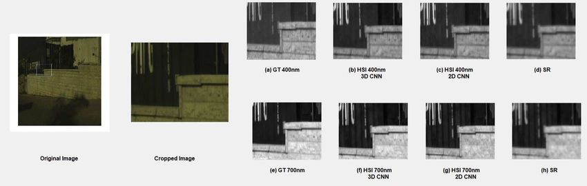
Figure 1. Comparison between RGB image and hypercube. Hypercube contains 3-dimensional data of a 2-dimensional image which are
captured on each wavelength The left most represent the spectral signature.The right most represents the RGB image intensity curve for
each pixel. Image reproduced from [26]

ized hardware based strategies is not physically possible. So         achieve on-par performance with state of art, we present 2D
various methods have been proposed to get fast and accurate           and 3D CNN architectures for reconstruction of spectral
hyperspectral images.                                                 data from RGB images. In [2] spectral reconstruction
   Computed       tomography       imaging     spectrometers          has been done using generative adversarial network. In
(CTIS)[11] [21] is used to construct 3D hyperspectral                 CNN, features are extracted from the image by convolving
data from 2D imaging sensor. The hyperspectral image can              kernels on the image, these kernels are updated using
be constructed by using multiplexed 2D data, but post pro-            various optimizers to construct the required features. In this
cessing and specialized hardware are required as a whole              paper, we explore application of both 2D and 3D kernels
to perform the operation. Due to sensor size limitation the           for spectral reconstruction from RGB image. A detailed
quality of hyperspectral images suffers in terms of spatial           comparison of the results obtained from application of
and spectral resolution. Recent advancement in the field              these kernels is also given. In the next section we will
of compressed sensing enhances the performance of CTIS                describe the problem of reconstructing spectral image from
in term of sensor utilization[8] [15] however, complex                RGB images.
acquisition and significant post processing still remains
bottleneck. Systems such as ”Hyperspectral fovea” [13]                2. Proposed Framework
etc. which are capable of acquiring high resolution RGB               2.1. Problem formulation
data, along with the spectral information of the central
image region in the image, are also proposed which acquire                In basic color science the conventional color images are
real time hyperspectral images without causing much                   formed by 3 channels i.e Red , Blue and Green which have
computational costs. These systems are mostly used in                 a strong dependency on the characteristics of imaging sys-
applications where occasional hyperspectral sampling area             tem that include the illuminance for image acquisition. Un-
are required rather than full hyperspectral cube. Matrix              like color images, spectral reflectance is proven to be the
factorization [22] method is used to construct hyperspectral          most accurate representation of the color of an object and it
data with high resolution with the help of RGB image and              is also completely independent of the imaging system. As
spectral images of low resolution. This methods produce               shown in Figure 1 hyperspectral image generally covers a
high estimation accuracy with high computation cost.                  common portion of visible spectrum with numerous spec-
Recent literature [?] [14] [16] [30] in hyperspectral shows           tral bands and higher spectral resolution than three-band
the researcher are estimating spectral values by using color          imaging (such as RGB images).
images(RGB).In recent years deep learning techniques                      The mapping between a hyperspectral reflectance spec-
have given effective and reliable performance for solving             trum and an RGB reflectance spectrum [25] for each pixel
non-linear problems. However, extraction of hyperspectral             at (x, y) can be modeled as[10] [35],
data from image using deep learning has not been explored                            µ3×1 = S3×N ∗ rN ×1 + e3×1                   (1)
extensively. The available literature [1] [14][2][42] showed
success of deep learning in constructing high resolution              where µ is a 3 × 1 vector that has RGB intensities, S is a
hyperspectral images with simply using color images and               3×N matrix of spectral responses of the three-color camera
their corresponding low resolution spectral images. In this           sensor, r is an N ×1 vector that has the reflectance intensity
paper, motivated by the potential of convolutional neural             normalized by the reflectance standard, and e is a 3 × 1
network (CNN) based architectures in [1] [42][2], which               vector of system noise with zero mean. N represents the

                                                                   958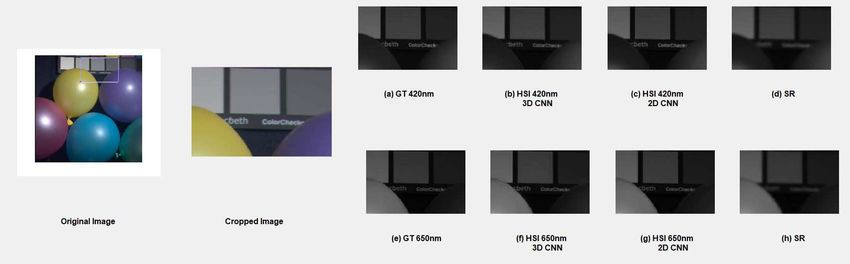
Figure 2. 2D-CNN proposed architecture

number of wavelengths. In general, S is obtained from the         to 700nm with every image at 10nm step. 2D-CNN model
sensor manufacturer or it can be estimated analytically by        as shown in Figure 2, having 2D kernel extracts the hyper-
training RGB samples [5] [34].                                    spectral information available in the spatial domain of the
    The goal is to predict r, reflectance vector, provided S      specific channel. The kernel convolves on individual chan-
and µ using equation 1. Please note that equation 1 belongs       nels and the average of the values generated for each pixel
to a system of linear equations and the dimension of S is         on these channels are considered. This technique efficiently
3 × N , so there exists an infinite number of solutions which     incorporates the spatial data however, an inter-channel co-
satisfy equation 1.                                               relation is left unnoticed and holds important information.
    Let us suppose, a color spectrum µ and respective re-         To incorporate the inter-channel co-relation we use 3D-
flectance spectrum r is collected for every sample, Xm×3          CNN as shown in Figure 3 with 3D kernel. A 3D kernel
and R̂m×N can be formed by organizing the spectra from            convolves in three dimensions, two spatial and one chan-
numerous independent samples, where N is the number of            nel, hence incorporates the related information between the
wavelength and m is the number of dissimilar samples. The         channels. Instead of simply averaging a 3D convolution op-
problem of reconstruction is supposed to learn conversion         eration adds up the response of all the corresponding pixels,
matrix T from the training set such that                          thus incorporating the correlated information.

                                                                  2.2. 2D-CNN
                 R̂n×N = Xm×3 ∗ T3×N                     (2)         Representation of RGB to hyperspectral conversion us-
                                                                  ing 2D-CNN is explained as follows:
   Relative absolute error can be used to compute T by min-
                                                                     Let X be the RGB input of dimension L × H × 3 and
imizing error between reconstructed spectra and original
                                                                  Y be the ground truth hyperspectral image of dimension
spectra. After computing T using training set, (reflectance
                                                                  L × H × 31, Here L is the length, H is height/width and 3
spectrum) can be estimated by using a RGB spectrum X as
                                                                  or 31 is channels. Input X is represented as C × L × H.
testing set.
                                                                  where C represent channel.
   The above formulation views the spectral reconstruction
                                                                     Feature Extraction: Feature extraction from input X is
from RGB images a linear problem. The frameworks used
                                                                  given by
in this work maps the nonlinear function from 3 channel
RGB to 31 channel hyperspectral image.                                     X1 = F1 (X) = max(0, X ∗ W1 + B1 )              (4)
                    Yn×N = F (Xm×3 )                     (3)         Here W1 contains n1 filters of size C × f1 × f1 and B1
                                                                  is n1 -dimensional vector.
where F is a non linear mapping between X and Y and
                                                                     The dimension of x1 is n1 ×L×H, ′ ∗′ is 2D convolution
Y ≈ R̂. Two frameworks have been proposed in this paper
                                                                  operator.
based on its kernel type. The first framework has 2D con-
                                                                     Non-Linear Mapping
volutional kernels and the second has 3D convolutional ker-
nels. The models are trained to extract the frequency based               X2 = F2 (X1 ) = max(0, X1 ∗ W2 + B2 )            (5)
information from the image. The last layer of the models
have 31 feature maps with every feature map having 10nm               Here W2 contains n2 filters of size n1 × f2 × f2 and B2
difference in wavelength from the consecutive feature. The        is n2 dimension vector. The dimension of X2 is n2 × L × H
input to these models are RGB images which have wave-
length between 400nm to 700nm and the ground truth have           XL−1 = FL−1 (XL−2 ) = max(0, XL−2 ∗ WL−1 + BL−1 )
thirty one images having wavelength starting from 400nm                                                       (6)

                                                                959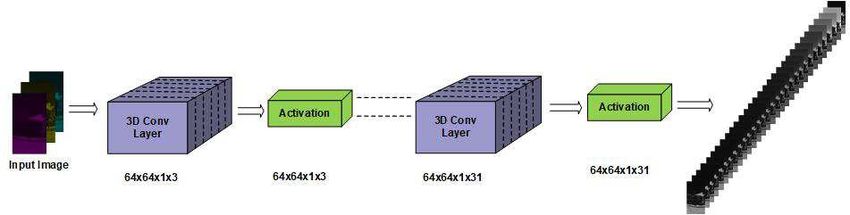
Figure 3. 3D-CNN proposed architecture

   Reconstruction: Reconstruction of hyperspectral im-           2.4. Training
ages is given by
                                                                     Individual models have been trained on distinct datasets
   XL = FL (XL−1 ) = max(0, XL−1 ∗ WL + BL )            (7)      [4][3][43]. We extracted the patches of size 64 × 64 × 3
Here WL is 31 filters of size fL ×fL and B2 is 31 dimension      from RGB input images and patches of size 64 × 64 × 31
vector. The dimension of XL will be 31 × L × H now the           are extracted from corresponding hyperspectral image. For
loss can be calculated by                                        NTIRE challenge, total number of training patches are
                                                                 84021. We trained a 5-layer architectures for both 2D
                   loss = ||Y − XL ||22                 (8)      and 3D CNN with learning rate of 10−4 with different
and we back propagate the gradient of loss to update the         hyper parameters. For training 3D-CNN, the channels of
weight and bias in each epoch.                                   the RGB image is considered as depth. To create such
                                                                 dataset, we split the channels of RGB and reshaped them in
2.3. 3D-CNN                                                      (height, width, 1) format followed by concatenating these
   We treat channels as depth by considering channel (c)         channels along third axis. This creates the data with the
= 1 and depth(d) = 3. Mathematical formulation of RGB            shape (height, width, 1, channels). Similar approach is
to hyperspectral conversion using 3D-CNN is modeled as           followed to create corresponding ground truth. Patches of
follows:                                                         size 64 × 64 are then extracted from this dataset. This data
   Let X be represented as of dimension c × d × L × H or         is then passed to the model as explained section 2.3 and
1 × d × L × H or d × L × H                                       section 2.4. The kernel size for both the models are 3 × 3
   Feature Extraction: Feature extraction from input X is        and 3 × 3 × 3 respectively. CNN performs exceptionally
given by                                                         well for non-linear problems, however selection of train-
                                                                 able parameters is quite a tedious task. The parameters are
         X1 = F1 (X) = max(0, X ⊗ W1 + B1 )             (9)      chosen using brute force cracking. Parameters giving opti-
   Here F represents the operation by a 3D kernel ’⊗’ is         mum results with less complexity are considered. To train
3D convolution operator and W1 contains n1 filters of size       the model we are using Adam optimizer and minimizing the
d1 xf1 xf1 or 1 × d1 × f1 × f1 , Here (∵d1 < d)                  mean absolute error between the model output and ground
   The dimension of X1 will be n1 × L × H.                       truth.
   Non-linear Mapping in Multiple Steps :
                                                                 2.5. Testing
      X2 = F2 (X1 ) = max(0, X1 ⊗ W2 + B2 )            (10)
                                                                    To test the model, learned model is inferred. Testing can
  Here W2 contain n2 filter of size d2 ×f2 ×f2 (∵d2 < n1 )
                                                                 be represented for both 2D-CNN and 3D-CNN model by.
                 XL−1 = FL−1 (XL12 )                   (11)
   Hence WL−1 contains nL−1 filter of size dL−1 ×fL−1 ×                               XL = GL (XL−1 )
f L − 1 (∵dL−1 ≤ nL−2 )
   Reconstruction:                                                                  = GL (FL−1 (XL−2 ))
   Reconstruction of hyperspectral images given by
         XL = FL (XL−1 ) = XL−1 ⊗ WL + BL              (12)                         = GL .FL−1 ......F1 (X)

   Here WL is 31 filter of size dL × fL × fL (∵dL ≤ nL−1 )
The dimension XL will be 31 × L × H Same the loss is                                    ∵ XL = G(X)                     (13)
calculated as by equation 3 and similarly the weights are
update by back propagating the gradient loss.                    where G represents both F and F.

                                                              960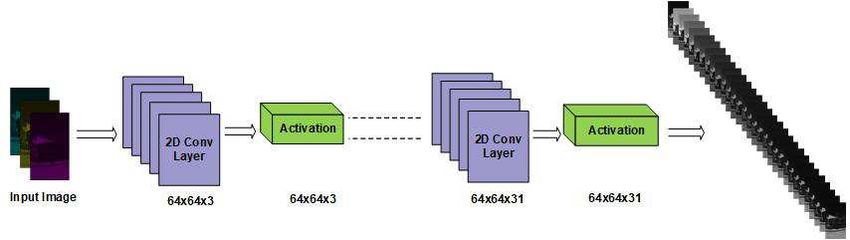
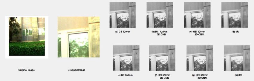
Figure 4. Hyperspectral image comparison on NTIRE-2018 dataset

                                   Figure 5. Hyperspectral image comparison on CAVE dataset

3. Experimental Results                                           it also consists of 31 spectral bands with range 400-700nm
                                                                  with 10nm steps.
   We implemented our algorithms using Keras and Ten-                 The iCVL dataset consists of 202 images taken by
sorflow, running on Intel Core i7 CPU at 3.6 GHz with 16          Specim DX4 hyperspectral camera. Each image is of size
GB RAM and Nvidia 8 GB GTX 1080 GPU. We evaluated                 1392 × 1300 × 31 spectral band images ranging from 400-
the proposed approach using the hyperspectral images from         700nm with 10nm steps.
NTIRE-2018[4], iCVL[3] and CAVE [43] databases. Root
Mean Square Error (RMSE), Mean Squared error(MSE)                 3.2. Result Analysis
and Mean Relative Absolute Error (MRAE) are used as
evaluation metrics. RMSE is useful in analyzing the re-
                                                                               Table 1. Results on NTIRE-2018 dataset
construction of individual spectral channels of the estimated
hyperspectral images and MRAE is sensitive to extreme val-                  Approach             RMSE     MRAE          Time (in seconds)
ues (i.e outliers) and to low values.                                        3D-CNN              20.010   0.018                 11
                                                                             2D-CNN              21.394   0.020                2.3
3.1. Datasets
                                                                             VIDAR1              14.45    0.0137               180
    2D-3D CNN model are tested and trained using NTIRE-                      VIDAR2              13.98    0.0137                96
2018 image dataset[4], CAVE [43] and iCVL dataset [3].                     HypedPhoti            16.07    0.0153                57
NTIRE-2018 dataset consists of of 254 hyperspectral im-                        LFB               16.19    0.0152                 -
ages captured by Specim PS Kappa DX4 camera with a ro-                     IVRL Prime            16.17    0.0155              170/2
tary stage for the spatial scanning. Out of 256 hyperspec-                     sr402             16.92    0.0164                12
tral images 201 images are taken from iCVL dataset [3].                        CVL               17.27    0.0174                 1
The size of provided images are 1392 × 1300 × 31 with 31                    advr gb3hs           24.81    0.0218                40
spectral channels in the range 400-700nm with 10nm steps.                    SPECR C             24.81    0.0401                 -
CAVE dataset consists 32 hyperspectral images taken by                sparse recovery(SR)[3]     24.03    0.056                  -
Apogee Alta U260 camera size of each image is512 × 512,

                                                                961
Figure 6. Hyperspectral image comparison on iCVL dataset
To illustrate the effectiveness of our proposed 2D & 3D Table 3. Results on iCVL dataset
Approach RMSE MSE
CNN based approach to convert RGB to hyperspectral im-
3D-CNN 1.115 0.0051
age, we have compared our techniques with other state-of-
2D-CNN 2.12 0.0086
the-art methods(Table 1, Table 2, Table 3). For evaluating
alvarez et. al[2] 1.457 -
performance of our techniques we have used mean relative
S.R[3] 2.56 -
absolute error (MRAE), root mean square error (RMSE),
A+ 1 × 1[1] 1.12 -
mean squared error(MSE) and run time per image.
A+ 3 × 3[1] 1.04 -
The results and comparison of methods from NTIRE-
2018 challenge can be seen from Table 1. The proposed
algorithms performs on par with other methods as can be
observed by comparing RMSE and MRAE in both of the
that our methods have very less run time requirement with
proposed methods with far less run time per image. We
the performance on par as compared to other methods pre-
have also shown the relative performance of the proposed
sented in the challenge. We have compared 2D and 3D ker-
methods compared to other CNN based algorithms in Table
nel based CNN for spectral reconstruction.
2 and Table 3 on CAVE and iCVL datasets respectively. As
can be seen Figure 4 the 400nm band and also in 700nm
band and Figure 5,Figure 6 for 420nm and 650 nm band References
3D-CNN reconstruction has preserved finer details as com-
[1] J. Aeschbacher, J. Wu, R. Timofte, D. CVL, and E. ITET. In
pared to sparse recovery (SR). It is also evident from Figure
defense of shallow learned spectral reconstruction from rgb
5,Figure 6 2D-CNN has also out performed sparse recovery images. In Proceedings of the IEEE Conference on Com-
(SR) method. puter Vision and Pattern Recognition, pages 471–479, 2017.
Table 2. Results on CAVE dataset [2] A. Alvarez-Gila, J. van de Weijer, and E. Garrote. Adversar-
Approach RMSE MSE ial networks for spatial context-aware spectral image recon-
3D-CNN 2.86 0.0065 struction from rgb. arXiv preprint arXiv:1709.00265, 2017.
2D-CNN 3.05 0.0075 [3] B. Arad and O. Ben-Shahar. Sparse recovery of hyperspec-
S.R[3] 5.40 - tral signal from natural rgb images. In European Conference
A+ 1 × 1[1] 2.74 - on Computer Vision, pages 19–34. Springer, 2016.
A+ 3 × 3[1] 2.90 - [4] B. Arad, O. Ben-Shahar, R. Timofte, L. Van Gool, L. Zhang,
M.-H. Yang, et al. Ntire 2018 challenge on spectral recon-
struction from rgb images. In The IEEE Conference on Com-
puter Vision and Pattern Recognition (CVPR) Workshops,
4. Conclusion June 2018.
[5] K. Barnard and B. Funt. Camera characterization for color
We have given a CNN based framework to reconstruct research. Color Research & Application, 27(3):152–163,
multiple spectral bands (Hyperspectral image) from three 2002.
spectral bands (RGB). Subsequently, we have shown that [6] E. Belluco, M. Camuffo, S. Ferrari, L. Modenese, S. Sil-
our CNN based deep learning model with minimal layer (5) vestri, A. Marani, and M. Marani. Mapping salt-marsh veg-
have outperformed the current traditional method of extract- etation by multispectral and hyperspectral remote sensing.
ing hyperspectral data from RGB images. It is also evident Remote sensing of environment, 105(1):54–67, 2006.
962[7] M. Borengasser, W. S. Hungate, and R. Watkins. Hyperspec- ing via matrix factorization. In Computer Vision and Pat-
tral remote sensing: principles and applications. CRC press, tern Recognition (CVPR), 2011 IEEE Conference on, pages
2007. 2329–2336. IEEE, 2011.
[8] D. J. Brady and M. E. Gehm. Compressive imaging spec- [23] Z. Khan, F. Shafait, and A. Mian. Automatic ink mismatch
trometers using coded apertures. In Visual Information Pro- detection for forensic document analysis. Pattern Recogni-
cessing XV, volume 6246, page 62460A. International Soci- tion, 48(11):3615–3626, 2015.
ety for Optics and Photonics, 2006. [24] S. J. Kim, F. Deng, and M. S. Brown. Visual enhancement of
[9] A. Castrodad, Z. Xing, J. Greer, E. Bosch, L. Carin, and old documents with hyperspectral imaging. Pattern Recog-
G. Sapiro. Discriminative sparse representations in hyper- nition, 44(7):1461–1469, 2011.
spectral imagery. In Image Processing (ICIP), 2010 17th [25] T. Kim, J.-I. Kim, M. A. V. Onufrak, C. Chapple, and Y. L.
IEEE International Conference on, pages 1313–1316. IEEE, Kim. Nonspectroscopic imaging for quantitative chlorophyll
2010. sensing. Journal of Biomedical Optics, 21(1):016008, 2016.
[10] S. Chen and Q. Liu. Modified wiener estimation of diffuse [26] G. Lu and B. Fei. Medical hyperspectral imaging: a review.
reflectance spectra from rgb values by the synthesis of new Journal of biomedical optics, 19(1):010901, 2014.
colors for tissue measurements. Journal of Biomedical op- [27] F. Melgani and L. Bruzzone. Classification of hyperspectral
tics, 17(3):030501, 2012. remote sensing images with support vector machines. IEEE
[11] M. Descour and E. Dereniak. Computed-tomography imag- Transactions on geoscience and remote sensing, 42(8):1778–
ing spectrometer: experimental calibration and reconstruc- 1790, 2004.
tion results. Applied Optics, 34(22):4817–4826, 1995. [28] P. J. Miller and C. C. Hoyt. Multispectral imaging with a liq-
[12] D. T. Dicker, J. Lerner, P. Van Belle, D. Guerry, 4th, M. Her- uid crystal tunable filter. In Optics in Agriculture, Forestry,
lyn, D. E. Elder, and W. S. El-Deiry. Differentiation of nor- and Biological Processing, volume 2345, pages 354–366. In-
mal skin and melanoma using high resolution hyperspectral ternational Society for Optics and Photonics, 1995.
imaging. Cancer biology & therapy, 5(8):1033–1038, 2006. [29] R. M. Nguyen, D. K. Prasad, and M. S. Brown. Training-
[13] D. W. Fletcher-Holmes and A. R. Harvey. Real-time imaging based spectral reconstruction from a single rgb image. In
with a hyperspectral fovea. Journal of Optics A: Pure and European Conference on Computer Vision, pages 186–201.
Applied Optics, 7(6):S298, 2005. Springer, 2014.
[14] S. Galliani, C. Lanaras, D. Marmanis, E. Baltsavias, and [30] M. Parmar, S. Lansel, and B. A. Wandell. Spatio-spectral
K. Schindler. Learned spectral super-resolution. arXiv reconstruction of the multispectral datacube using sparse re-
preprint arXiv:1703.09470, 2017. covery. In Image Processing, 2008. ICIP 2008. 15th IEEE
[15] M. Gehm, R. John, D. Brady, R. Willett, and T. Schulz. International Conference on, pages 473–476. IEEE, 2008.
Single-shot compressive spectral imaging with a dual- [31] L. L. Randeberg, I. Baarstad, T. Løke, P. Kaspersen, and
disperser architecture. Optics express, 15(21):14013–14027, L. O. Svaasand. Hyperspectral imaging of bruised skin.
2007. In Photonic Therapeutics and Diagnostics II, volume 6078,
[16] M. Goel, E. Whitmire, A. Mariakakis, T. S. Saponas, page 60780O. International Society for Optics and Photon-
N. Joshi, D. Morris, B. Guenter, M. Gavriliu, G. Borriello, ics, 2006.
and S. N. Patel. Hypercam: hyperspectral imaging for ubiq- [32] R. Richter and D. Schläpfer. Geo-atmospheric process-
uitous computing applications. In Proceedings of the 2015 ing of airborne imaging spectrometry data. part 2: atmo-
ACM International Joint Conference on Pervasive and Ubiq- spheric/topographic correction. International Journal of Re-
uitous Computing, pages 145–156. ACM, 2015. mote Sensing, 23(13):2631–2649, 2002.
[17] A. F. Goetz, G. Vane, J. E. Solomon, and B. N. Rock. [33] A. Robles-Kelly. Single image spectral reconstruction for
Imaging spectrometry for earth remote sensing. Science, multimedia applications. In Proceedings of the 23rd ACM
228(4704):1147–1153, 1985. international conference on Multimedia, pages 251–260.
[18] R. O. Green, M. L. Eastwood, C. M. Sarture, T. G. Chrien, ACM, 2015.
M. Aronsson, B. J. Chippendale, J. A. Faust, B. E. Pavri, [34] H.-L. Shen and J. H. Xin. Spectral characterization of a color
C. J. Chovit, M. Solis, et al. Imaging spectroscopy and the scanner by adaptive estimation. JOSA A, 21(7):1125–1130,
airborne visible/infrared imaging spectrometer (aviris). Re- 2004.
mote sensing of environment, 65(3):227–248, 1998. [35] H.-L. Shen, J. H. Xin, and S.-J. Shao. Improved reflectance
[19] S. Hwang, J. Park, N. Kim, Y. Choi, and I. S. Kweon. Mul- reconstruction for multispectral imaging by combining dif-
tispectral pedestrian detection: Benchmark dataset and base- ferent techniques. Optics express, 15(9):5531–5536, 2007.
line. Integrated Comput.-Aided Eng, 20:347–360, 2013. [36] G. N. Stamatas, C. J. Balas, and N. Kollias. Hyperspectral
[20] J. James. Spectrograph design fundamentals. Cambridge image acquisition and analysis of skin. In Spectral Imag-
University Press, 2007. ing: Instrumentation, Applications, and Analysis II, volume
[21] W. R. Johnson, D. W. Wilson, and G. Bearman. Spatial- 4959, pages 77–83. International Society for Optics and Pho-
spectral modulating snapshot hyperspectral imager. Applied tonics, 2003.
optics, 45(9):1898–1908, 2006. [37] S. Tominaga. Multichannel vision system for estimating sur-
[22] R. Kawakami, Y. Matsushita, J. Wright, M. Ben-Ezra, Y.- face and illumination functions. JOSA A, 13(11):2163–2173,
W. Tai, and K. Ikeuchi. High-resolution hyperspectral imag- 1996.
963[38] E. Underwood, S. Ustin, and D. DiPietro. Mapping nonna-
tive plants using hyperspectral imagery. Remote Sensing of
Environment, 86(2):150–161, 2003.
[39] M. Uzair, A. Mahmood, and A. Mian. Hyperspectral
face recognition with spatiospectral information fusion and
pls regression. IEEE Transactions on Image Processing,
24(3):1127–1137, 2015.
[40] M. Uzair, A. Mahmood, and A. S. Mian. Hyperspectral face
recognition using 3d-dct and partial least squares. In BMVC,
2013.
[41] H. Van Nguyen, A. Banerjee, and R. Chellappa. Track-
ing via object reflectance using a hyperspectral video cam-
era. In Computer Vision and Pattern Recognition Work-
shops (CVPRW), 2010 IEEE Computer Society Conference
on, pages 44–51. IEEE, 2010.
[42] Z. Xiong, Z. Shi, H. Li, L. Wang, D. Liu, and F. Wu. Hscnn:
Cnn-based hyperspectral image recovery from spectrally un-
dersampled projections. In Proceedings of the IEEE Interna-
tional Conference on Computer Vision Workshops, volume 2,
2017.
[43] F. Yasuma, T. Mitsunaga, D. Iso, and S. K. Nayar. General-
ized assorted pixel camera: postcapture control of resolution,
dynamic range, and spectrum. IEEE transactions on image
processing, 19(9):2241–2253, 2010.
[44] D. Zhang, W. Zuo, and F. Yue. A comparative study of
palmprint recognition algorithms. ACM computing surveys
(CSUR), 44(1):2, 2012.
[45] Y. Zhao and R. S. Berns. Image-based spectral reflectance
reconstruction using the matrix r method. Color Research &
Application, 32(5):343–351, 2007.
964You can also read


