A comprehensive empirical analysis on cross-domain semantic enrichment for detection of depressive language
←
→
Page content transcription
If your browser does not render page correctly, please read the page content below
A comprehensive empirical analysis on cross-domain semantic enrichment for
                                                                detection of depressive language

                                                                         Nawshad Farruque, Randy Goebel and Osmar Zaı̈ane
                                                                                            Department of Computing Science
                                                                                                  University of Alberta
                                                                                               Alberta, T6G 2E8, Canada
arXiv:2106.12797v1 [cs.CL] 24 Jun 2021

                                                                     Abstract                                 through suicide each year worldwide1 . Moreover, the eco-
                                                                                                              nomic burden created by depression is estimated to have
                                           We analyze the process of creating word embedding feature          been 210 billion USD in 2010 in the USA alone (Green-
                                           representations designed for a learning task when annotated        berg et al. 2015). Hence, detecting, monitoring and treating
                                           data is scarce, for example, in depressive language detec-         depression is very important and there is huge need for effec-
                                           tion from Tweets. We start with a rich word embedding pre-         tive, inexpensive and almost real-time interventions. In such
                                           trained from a large general dataset, which is then augmented
                                           with embeddings learned from a much smaller and more spe-
                                                                                                              a scenario, social media, such as, Twitter and Facebook, pro-
                                           cific domain dataset through a simple non-linear mapping           vide the foundation of a remedy. Social media are very pop-
                                           mechanism. We also experimented with several other more            ular among young adults, where depression is prevalent. In
                                           sophisticated methods of such mapping including, several           addition, it has been found that people who are otherwise
                                           auto-encoder based and custom loss-function based meth-            socially aloof (and more prone to having depression) can be
                                           ods that learn embedding representations through gradually         very active in the social media platforms (De Choudhury et
                                           learning to be close to the words of similar semantics and         al. 2013b). As a consequence, there has been significant de-
                                           distant to dissimilar semantics. Our strengthened representa-      pression detection research, based on various social media
                                           tions better capture the semantics of the depression domain,       attributes, such as social network size, social media behav-
                                           as it combines the semantics learned from the specific do-         ior, and language used in social media posts. Among these
                                           main coupled with word coverage from the general language.
                                           We also present a comparative performance analyses of our
                                                                                                              multi-modalities, human language alone can be a very good
                                           word embedding representations with a simple bag-of-words          predictor of depression (De Choudhury et al. 2013b). How-
                                           model, well known sentiment and psycholinguistic lexicons,         ever, the main bottle neck of social media posts-based de-
                                           and a general pre-trained word embedding. When used as             pression detection task is the lack of labelled data to identify
                                           feature representations for several different machine learn-       rich feature representations, which provide the basis for con-
                                           ing methods, including deep learning models in a depressive        structing models that help identify depressive language.
                                           Tweets identification task, we show that our augmented word
                                           embedding representations achieve a significantly better F1           Here we discuss the creation of a word embedding that
                                           score than the others, specially when applied to a high qual-      leverages both the Twitter vocabulary (from pre-trained
                                           ity dataset. Also, we present several data ablation tests which    Twitter word embedding) and depression semantics (from
                                           confirm the efficacy of our augmentation techniques.               a word embedding created from depression forum posts) to
                                                                                                              identify depressive Tweets. We believe our proposed meth-
                                                                                                              ods would significantly relieve us from the burden of curat-
                                                                 Introduction                                 ing a huge volume of human annotated data / high quality
                                                                                                              labelled data (which is very expensive and time consuming)
                                         Depression or Major Depressive Disorder (MDD) is re-                 to support the learning of better feature representations, and
                                         garded as one of the most commonly identified mental health          eventually lead to improved classification. In the next sec-
                                         problems among young adults in developed countries, ac-              tions we provide a brief summary of earlier research together
                                         counting for 75% of all psychiatric admissions (Boyd et              with some background supporting our formulation of our
                                         al. 1982). Most people who suffer from depression do not             proposed methods for identifying depression from Tweets.
                                         acknowledge it, for various reasons, ranging from social
                                         stigma to plain ignorance; this means that a vast majority             Throughout our paper, we use the phrase “word embed-
                                         of depressed people remain undiagnosed. Lack of diagno-              ding” as an object that consists of word vectors. So by “word
                                         sis eventually results in suicide, drug abuse, crime and many        embeddings” we mean multiple instances of that object.
                                         other societal problems. For example, depression has been
                                         found to be a major cause behind 800,000 deaths committed
                                                                                                                1
                                         Copyright © 2019, Association for the Advancement of Artificial          https://who.int/mental_health/prevention/
                                         Intelligence (www.aaai.org). All rights reserved.                    suicide/suicideprevent/en/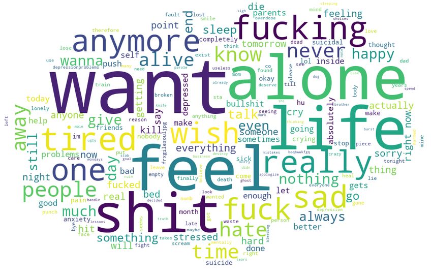
Background & motivation                              prerequisite for accurately identifying depression at the user
Previous studies suggest that the words we use in our daily        level (De Choudhury 2013a). In addition, most of this ear-
life can express our mental state, mood and emotion (Pen-          lier research leveraged Twitter posts to identify depression
nebaker, Mehl, and Niederhoffer 2003). Therefore analyzing         because a huge volume of Twitter posts are publicly avail-
language to identify and monitor human mental health prob-         able.
lems has been regarded as an appropriate avenue of mental             Therefore the motivation of our research comes from the
health modeling. With the advent of social media platforms,        need for a better feature representation specific to depressive
researchers have found that social media posts can be used as      language, and reduced dependency on a large set of (human
a good proxy for our day to day language usage (De Choud-          annotated) labelled data for depressive Tweet detection task.
hury et al. 2013b). There have been many studies that iden-        We proceed as follows:
tify and monitor depression through social media posts in          1. We create a word embedding space that encodes the se-
various social media, such as, Twitter (Reece et al. 2017;            mantics of depressive language from a small but high
De Choudhury 2013a; De Choudhury et al. 2013b), Face-                 quality depression corpus curated from depression related
book (Schwartz et al. 2014; Moreno et al. 2011) and online            public forums.
forums (Yates, Cohan, and Goharian 2017).
   Depression detection from social media posts can be spec-       2. We use that word embedding to create feature representa-
ified as a low resource supervised classification task be-            tions for our Tweets and feed them to our machine learn-
cause of the paucity of valid data. Although there is no              ing models to identify depressive Tweets; this achieves
concrete precise definition of valid data, previous research          good accuracy, even with very small amount of labelled
emphasizes collecting social media posts, which are ei-               Tweets.
ther validated by annotators as carrying clues of depres-          3. Furthermore, we adjust a pre-trained Twitter word embed-
sion, or coming from the people who are clinically diag-              ding based on our depression specific word embedding,
nosed as depressed, or both. Based on the methods of de-              using a non-linear mapping between the embeddings (mo-
pression intervention using these data, earlier research can          tivated by the work of (Mikolov, Le, and Sutskever 2013b)
be mostly divided into two categories: (1) general categories         and (Smith et al. 2017) on bilingual dictionary induction
of post-specific depression detection (or depressive lan-             for machine translation), and use it to create feature rep-
guage detection) (De Choudhury 2013a; Jamil et al. 2017;              resentation for our Tweets and feed them to our machine
Vioulès et al. 2018), and (2) user-specific depression detec-        learning models. This helps us achieve 4% higher F1-
tion, which considers all the posts made by a depressed user          score than our strongest baseline in depressive Tweets de-
in a specific time window (Resnik, Garron, and Resnik 2013;           tection.
Resnik et al. 2015). The goal of (1) is to identify depression
in a more fine grained level, i.e., in social media posts, which      Accuracy improvements mentioned in points 2 and 3
further helps in identifying depression inclination of individ-    above are true for a high quality dataset curated through
uals when analyzed by method (2).                                  rigorous human annotation, as opposed to the low quality
   For the post specific depression detection task, previous       dataset with less rigorous human annotation; this indicates
research concentrate on the extraction of depression spe-          the effectiveness of our proposed feature representations for
cific features used to train machine learning models, e.g.,        depressive Tweets detection. To the best of our knowledge,
building depression lexicons based on unigrams present             ours is the first effort to build a depression specific word
in posts from depressed individuals (De Choudhury et al.           embedding for identifying depressive Tweets, and to formu-
2013b), depression symptom related unigrams curated from           late a method to gain further improvements on top of it, then
depression questionnaires (Cheng et al. 2016), metaphors           to present a comprehensive analysis on the quantitative and
used in depressive language (Neuman et al. 2012), or psy-          qualitative performance of our embeddings.
cholinguistic features in LIWC (Tausczik and Pennebaker
2010). For user specific depression identification, variations                              Datasets
of topic modeling have been popular to identify depres-
                                                                   Here we provide the details of our two datasets that we use
sive topics and use them as features (Resnik et al. 2015;
                                                                   for our experiments and their annotation procedure, the cor-
Resnik, Garron, and Resnik 2013). But recently, some re-
                                                                   pus they are curated from and their quality comparisons.
search has used convolutional neural network (CNN) based
deep learning models to learn feature representations (Yates,
Cohan, and Goharian 2017) and (Orabi et al. 2018). Most            Dataset1
deep learning approaches require a significant volume of la-       Dataset1 is curated by the ADVanced ANalytics for data Sci-
belled data to learn the depression specific embedding from        encE (ADVANSE) research team at the University of Mont-
scratch, or from a pre-trained word embedding in a super-          pellier, France (Vioulès et al. 2018). This dataset contains
vised manner. So, in general, both post level and user level       Tweets having key-phrases generated from the American
depression identification research emphasize the curation of       Psychiatric Association (APA)’s list of risk factors and the
labelled social media posts indicative of depression, which        American Association of Suicidology (AAS)’s list of warn-
is a very expensive process in terms of time, human effort,        ing signs related to suicide. Furthermore, they randomly in-
and cost. Moreover, previous research showed that a robust         vestigated the authors of these Tweets to identify 60 dis-
post level depression identification system is an important        tressed users who frequently write about depression, suicide
and self mutilation. They also randomly collected 60 con- Tweets may convey depression as well; (5) they identified
trol users. Finally, they curated a balanced and human an- a person is depressed if s/he disclose their depression, but
notated dataset of a total of around 500 Tweets, of which they did not mention how they determined these disclosures.
50% Tweets are from distressed and 50% are from control Simple regular expression based methods to identify these
users, with the help of seven annotators and one professional self disclosures can introduce a lot of noise in the data. In
psychologist. The goal of their annotation was to provide a addition, these self disclosures may not be true.
distress score (0 - 3) for each Tweet. They reported a Co-
hen’s kappa agreement score of 69.1% for their annotation
task. Finally, they merged Tweets showing distress level 0, 1 Analysis based on linguistic components present in the
as control Tweets and 2, 3 as distressed Tweets. Distressed dataset: For this analysis, we use Linguistic Inquiry and
Tweets carry signs of suicidal ideation, self-harm and de- Word Count (LIWC) (Tausczik and Pennebaker 2010).
pression while control Tweets are about daily life occur- LIWC is a tool widely used in psycholinguistic analysis of
rences, such as weekend plans, trips and common distress language. It extracts the percentage of words in a text, across
such as exams, deadlines, etc. We believe this dataset is per- 93 pre-defined categories, e.g., affect, social process, cogni-
fectly suited for our task, and we use their distressed Tweets tive processes, etc. To analyse the quality of our datasets,
as our depressive Tweets and their control as our control. we provide scores of few dimensions of LIWC lexicon rele-
vant for depressive language detection (Nguyen et al. 2014),
Dataset2 (De Choudhury et al. 2013b) and (Kuppens et al. 2012), such
as, 1st person pronouns, anger, sadness, negative emotions,
Dataset2 is collected by a research group at the University etc, see Table 1 for the depressive Tweets present both in
of Ottawa (Jamil et al. 2017). They first filtered depressive our datasets. The bold items in that table shows significant
Tweets from #BellLetsTalk2015 (a Twitter campaign) based score differences in those dimensions for both datasets and
on keywords such as, suffer, attempt, suicide, battle, strug- endorses the fact that Dataset1 indeed carries more linguis-
gle and first person pronouns. Using topic modeling, they re- tic clues of depression than Dataset2 (the higher the score,
moved Tweets under the topics of public campaign, mental the more is the percentage of words from that dimension is
health awareness, and raising money. They further removed present in the text). Moreover, Tweets labelled as depressive
Tweets which contain mostly URLs and are very short. Fi- in Dataset2 are mostly about common distress of everyday
nally, from these Tweets they identified 30 users who self- life unlike those of Dataset1, which are indicative of severe
disclosed their own depression, and 30 control users who did depression. Figures 1 and 2 depict the word clouds created
not. They employed two annotators to label Tweets from 10 from Dataset1 and Dataset2 depressive Tweets respectively.
users as either depressed or non-depressed. They found that We provide few random samples of Tweets from Dataset1
their annotators labelled most Tweets as non-depressed. To and Dataset2 at Table 2 as well.
reduce the number of non-depressive Tweets, they further
removed neutral Tweets from their dataset, as they believe
neutral Tweets surely do not carry any signs of depression. Dataset1 Dataset2
LIWC Example
After that, they annotated Tweets from the remaining 50 Depressive Depressive
Category Words
users with the help of two annotators with a Cohen’s kappa Tweets score Tweets score
agreement score of 67%. Finally, they labelled a Tweet as 1st person
I, me, mine 12.74 7.06
depressive if any one of their two annotators agree, to gather pronouns
no, not,
more depressive Tweets. This left them with 8,753 Tweets Negations 3.94 2.63
never
with 706 depressive Tweets. Positive love, nice,
2.79 2.65
Emotion sweet
Quality of Datasets Negative hurt, ugly,
8.59 6.99
Here we present a comparative analysis of our datasets Emotion nasty
based on their curation process and the linguistic compo- worried,
Anxiety 0.72 1.05
nents present in them relevant to depressive language detec- fearful
tion as follows: hate, kill,
Anger 2.86 2.51
annoyed
Analysis based on data curation process: We think crying, grief,
Sadness 3.29 1.97
Dataset2 is of lower quality compared to Dataset1 for the sad
following reasons: (1) this dataset is collected from the pool ago, did,
Past Focus 2.65 3
of Tweets which is a part of a mental health campaign, and talked
thus compromises the authenticity of the Tweets; (2) the suicide, die,
Death 1.43 0.44
overdosed
words they used for searching depressive Tweets are not val-
fuck, damn,
idated by any depression or suicide lexicons; (3) although Swear 1.97 1.39
shit
they used two annotators (none of them are domain experts)
to label the Tweets, they finally considered a Tweet as de- Table 1: Score of Dataset1 and Dataset2 in few LIWC di-
pressive if at least one annotator labelled it as depressive, mensions relevant to depressive language detection
hence introduced more noise in the data; (4) it is not con-
firmed how they identified neutral Tweets since their neutralsive Tweets identification, so our datasets are from Twitter,
not from depression forums. We are using depression forum
posts only to learn improved word embedding feature rep-
resentation that can help us identifying depressive Tweets in
the above mentioned Twitter datasets.
Creating a depression specific corpus
To build a depression specific word embedding, we curate
our own depression corpus. For this, we collect all the posts
from the Reddit depression forum: r/depression 2 between
Figure 1: Dataset1 depressive Tweets word cloud
2006 to 2017 and all those from Suicidal Forum 3 and con-
catenated for a total of 856,897 posts. We choose these fo-
rums because people who post anonymously in these fo-
rums usually suffer from severe depression and share their
struggle with depression and its impact in their personal
lives (De Choudhury and De 2014). We believe these forums
contain useful semantic components indicative of depressive
language.
Feature extraction methods
Bag-of-Words (BOW)
Figure 2: Dataset2 depressive Tweets word cloud We represent each Tweet as a vector of vocabulary terms and
their frequency counts in that Tweet, also known as bag-of-
words. The vocabulary terms refer to the most frequent 400
Datasets Depressive Tweets
terms existing in the training set. Before creating the vocabu-
Dataset1 “I wish I could be normal and be happy and feel
things like other people”
lary and the vector representation of the Tweets, we perform
“I feel alone even when I’m not” the following preprocessing: (1) we make the Tweets all
“Yesterday was difficult...and so is today and to- lowercase, then (2) tokenize them using the NLTK Tweet to-
morrow and the days after...” kenizer 4 ; the reason for using Tweet tokenizer is to consider
Dataset2 “Last night was not a good night for sleep... so Tweet emoticons (:-)), hashtags (#Depression) and mentions
tired And I have a gig tonight... yawnnn” (@user) as single tokens; we then (3) remove all stop words
“So tired of my @NetflixCA app not working, except the first person pronouns such as, I, me and my (be-
I hate Android 5” cause they are useful for depression detection) and then (4)
“I have been so bad at reading Twitter lately, I use NLTK porter stemmer 5 . Stemming helps us reduce spar-
don’t know how people keep up, maybe today sity of the bag-of-words representations of Tweets.
I’ll do better”
Table 2: Sample Tweets from Dataset1 and Dataset2
Lexicons
We experimented with several emotion and sentiment lex-
icons, such as, LabMT (Dodds et al. 2011), Emolex
Why these two datasets? (Mohammad and Turney 2013), AFINN (Nielsen 2011),
LIWC (Tausczik and Pennebaker 2010), VADER (Gilbert
We believe these two datasets represent the two broad cate-
2014), NRC-Hashtag-Sentiment-Lexicon (NHSL) (Kir-
gories of publicly available Twitter datasets for the depres-
itchenko, Zhu, and Mohammad 2014), NRC-Hashtag-
sive Tweets identification task. One category relies on key-
Emotion-Lexicon (NHEL) (Mohammad and Kiritchenko
words related to depression and suicidal ideation to identify
2015) and CBET (Shahraki and Zaı̈ane 2017). Among these
depressive Tweets and employed rigorous annotation to fil-
lexicons we find LIWC and NHEL perform the best and
ter out noisy Tweets (like Dataset1); the other relies on self
hence we report the results of these two lexicons. The fol-
disclosures of Twitter users to identify depressive Tweets
lowing subsections provide a brief description of LIWC,
and employed less rigorous annotation (like Dataset2) to fil-
NHEL and lexicon-based representation of Tweets.
ter noisy Tweets. So any other datasets that fall into one of
above categories or do not go through annotation procedure Linguistic Inquiry and Word Count (LIWC): LIWC
atleast like Dataset2, such as datasets released in a CLPsych has been widely used as a good baseline for depressive
2015 shared task (Coppersmith et al. 2015a) are not evalu- Tweet detection in earlier research (Nguyen et al. 2014;
ated in this research. Moreover, our Dataset2 is a represen-
2
tative of imbalanced dataset (with fewer depressive Tweets reddit.com/r/depression/
3
than non-depressive Tweets) which is a very common char- suicideforum.com/
4
acteristic of the datasets for depressive Tweets identification nltk.org/api/nltk.tokenize.html
5
task. It is also to be noted that we are interested in depres- nltk.org/_modules/nltk/stem/porter.htmlCoppersmith, Dredze, and Harman 2014). We use it to con- Even if we create one, there is a good chance that its vo-
vert a Tweet into a fixed length vector representation of 93 cabulary would be limited. Also, most importantly, there
dimensions, that is then used as the input for our machine is no comprehensive discussion/analysis in their paper on
learning models. how to retrofit those words which are only present in pre-
trained embedding but not in semantic lexicons or out-of-
NRC Hashtag Emotion Lexicon (NHEL): In NHEL vocabulary (OOV) words. In our method we do not depend
there are 16,862 unigrams, each of which are associated on any such semantic lexicons. We retrofitted a general pre-
with a vector of 8 scores for 8 emotions, such as, anger, trained embedding based on the semantics present in depres-
anticipation, disgust, fear, joy, sadness, surprise and trust. sion specific embedding through a non-linear mapping be-
Each of the scores (a real value between 0 and ∞) indicate tween them. Our depression specific embedding is created
how much a particular unigram is associated with each of in an unsupervised manner from depression forum posts.
the 8 emotions. In our experiments, we tokenize each Tweet Moreover, through our mapping process we learn a trans-
as described in the Bag-of-Words (BOW) section, then we formation matrix, see Equation 3, that can be further used
use the lexicon to determine a score for each token in the to predict embedding for OOVs and this helps us to achieve
Tweet; finally, we sum them to get a vector of 8 values for better accuracy (see Table 10).
each Tweet, which represents the expressed emotions in that Interestingly, there have been no attempts taken in depres-
tweet and their magnitude. Finally, we use that value as a sive language detection research area which primarily focus
feature for our machine learning models. on building better depression specific embedding in an un-
supervised manner, then further analyse its use in augment-
Distributed representation of words ing a general pre-trained embedding. Very recently (Orabi
Distributed representation of words (also known as word et al. 2018) proposed a multi-task learning method which
embedding (WE) or a collection of word vectors (Mikolov learns an embedding in a purely supervised way by si-
et al. 2013a)) capture the semantic and syntactic similarity multaneously performing (1) adjacent word prediction task
between a word and its context defined by its neighbour- from one of their labelled train dataset and (2) depres-
ing words that appear in a fixed window, and has been suc- sion/PTSD sentence prediction task again from the same
cessfully used as a compact feature representation in many labelled train dataset, where this labelled dataset was cre-
downstream NLP tasks. Previous research show that a do- ated with the help of human annotation. We have no such
main specific word embedding is usually better for perform- dependency on labelled data. Also, we have disjoint sets
ing domain specific tasks than a general word embedding, of data for learning/adjusting our embedding and detecting
e.g., (Bengio and Heigold 2014) proposed word embed- depressive Tweets across all our experiments, unlike them,
ding for speech recognition, (Tang et al. 2014) proposed the which makes our experiments fairer than theirs. They did not
same for sentiment classification and (Asgari and Mofrad provide any experimental result and analysis on depressive
2015) for representing biological sequences. Inspired by post (or Tweet) identification rather on depressive Twitter
these works, we here report the construction of depression user identification which is fundamentally different from our
specific word embedding, in an unsupervised manner, In ad- task. Also, our paper discusses the transferability of depres-
dition, we report that the word embedding resulting from a sive language specific semantics from forums to microblogs,
non-linear mapping between general (pre-trained) word em- which is not the focus of their paper. Finally, we argue that
bedding and depression specific word embedding can be a the dataset they used for depression detection is very noisy
very useful feature representation for our depressive Tweet and thus not very suitable for the same (See “Quality of
identification task. Datasets” section).
Our embedding adjustment method has some similarity In the following subsections we describe different word
to embedding retrofitting proposed by (Faruqui et al. 2015) embeddings used in our experiments.
and embedding refinement proposed by (Yu et al. 2018),
in the sense that we also adjusted (or retrofitted) our pre- General Twitter word Embedding (TE): We use a pre-
trained embedding. However, there is a major difference trained 400 dimensional skip-gram word embedding learned
between their method and ours. They only adjusted those from 400 million Tweets with vocabulary size of 3, 039, 345
words, w ∈ V , where V is the common vocabulary between words (Godin et al. 2015) as a representative of word em-
their pre-trained embedding and semantic/sentiment lexi- bedding learned from a general dataset (in our case, Tweets);
cons, e.g. WordNet (Miller 1995), ANEW (Nielsen 2011) we believe this captures the most relevant vocabulary for our
etc. By this adjustment they brought each word in the pre- task. The creator of this word embedding used negative sam-
trained embedding closer to the other words which are se- pling (k = 5) with a context window size = 1 and mincount
mantically related to them (as defined in the semantic lex- = 5. Since it is pre-trained, we do not have control over the
icons) through an iterative update method, where all these parameters it uses and simply use it as is.
words are member of V . So their method strictly depends
on semantic lexicons and their vocabularies. In depression Depression specific word Embedding (DE): We create a
detection research, where labelled data is scarce and hu- 400 dimensional depression specific word embedding (DE)
man annotation is expensive, building depression lexicons on our curated depression corpus. First, we identify sentence
(given there is no good publicly available depression lex- boundaries in our corpora based on punctuation, such as:
icons) and using them for retrofitting is counter intuitive. “?”,“!” and “.”. We then feed each sentence into a skip-grambased word2vec implementation in gensim 6 . We use nega- ATE original (ATE(orig.)): We report our general Twit-
tive sampling (k = 5) with the context window size = 5 and ter embedding (TE) adjusted by DE(original) or DE(orig.)
mincount = 10 for the training of these word embeddings. and we name it adjusted Twitter embedding, ATE(original)
DE has a vocabulary size of 29, 930 words. We choose skip- or ATE(orig.). DE(orig.) is created with same parameter set-
gram for this training because skip-gram learns good em- tings as our TE. We show that our DE with more frequent
bedding from a small corpus (Mikolov et al. 2013c). words (trained with mincount=10) and a bit larger context
(context window size=5) help us create an improved ATE.
Adjusted Twitter word Embedding (ATE): a non-linear A summary of the vocabulary sizes and the corpus our
mapping between TE and DE: In this step, we create a embedding sets are built on is provided in Table 3.
non-linear mapping between TE and DE. To do this, we use
a Multilayer Perceptron Regressor (MLP-Regressor) with a Word
single hidden layer with 400 hidden units and Rectified Lin- Corpus Type #Posts Vocab. Size
Embeddings
ear Unit (ReLU) activations (from hidden to output layer), TE, ATE and
Twitter 400M 3M
which attempts to minimize the Minimum Squared Error ATE (orig.)
(MSE) loss function, F(θ) in Equation 1, using stochastic DE
Depression
1.5M 30K
gradient descent: Forums
Table 3: Corpus and vocabulary statistics for word embed-
F(θ) = arg min(L(θ)) (1)
θ dings
where
m
1 X Conditions for embedding mapping/adjustment: Our
L(θ) = ||gi (x) − yi ||22 (2) non-linear mapping between two embeddings works better
m i=1
given that those two embeddings are created from the same
and word embedding creation algorithm (in our case skip-gram)
g(x) = ReLU (b1 + W1 (b2 + W2 x)) (3) and have same number of dimensions (i.e. 400). We also find
that a non-linear mapping between our TE and DE produces
here, g(x) is the non-linear mapping function between the slightly better ATE than a linear mapping for our task, al-
vector x (from TE) and y (from DE) of a word w ∈ V , though the former is a bit slower.
where, V is a common vocabulary between TE and DE; W1
and W2 are the hidden-to-output and input-to-hidden layer Other embedding augmentation methods:
weight matrices respectively, b1 is the output layer bias vec- We experiment with two more embedding augmentation
tor and b2 is the hidden layer bias vector (all these weights methods. These methods are actually a slightly complex ex-
and biases are indicated as θ in Equation 1) In Equation 2, tensions of our proposed methods and do not necessarily sur-
m is the length of V (in our case it is 28,977). Once the pass them in accuracy, hence we did not report them in our
MLPR learns the θ that minimizes F(θ), it is used to pre- ‘Results Analysis’ section, rather discuss here briefly.
dict the vectors for the words in TE which are not present
in DE (i.e., out of vocabulary(OOV) words for DE). After ATE-Centroids: We propose two more methods of em-
this step, we finally get an adjusted Twitter word embedding bedding augmentation which can be seen as an extension
which encodes the semantics of depression forums as well to our ATE construction method. In general, we call these
as word coverage from Tweets. We call these embedding the methods ATE-Centroids. For a word w ∈ V , where V is the
Adjusted Twitter word Embedding (ATE). The whole pro- common vocabulary between TE and DE. We learn a non-
cess is depicted in Figure 3. linear mapper (like the one we use to create ATE) which
does the following, (1) it learns to minimize the squared eu-
Prediction Phase clidean distance between the embedding of w in TE and the
Learned Non-linear Adjusted Twitter word
centroid (or average of word vectors) calculated from w and
Mapper Function Embedding (ATE) its neighbours in DE (i.e. the words which are close to it
in Euclidean distance in DE), we name the resulting em-
bedding from this method, ATE-Centroid-1. (2) along with
General Twitter word Embedding Minimizing squared Euclidean distance between embeddings,
(TE) thus mapping from TE to DE (Learning Phase) (1), it learns to maximize the distance between w in TE and
Common
Vocabulary, V
Non-linear Mapper Function
(MLP-Regressor)
the centroid calculated from the word vectors of the distant
Depression specific word
words from w in DE, we name the resulting embedding from
Embedding (DE)
this method, ATE-Centroid-2. After learning, the mapper is
used to predict OOV words (the words which are in TE but
Figure 3: Non-linear mapping of TE to DE (creation of not in DE). So in summary, by doing operations (1) and (2),
ATE) we basically adjust a source pre-trained embedding (in our
case TE) by pushing its constituent words close to the words
of close semantics and away from the words of distant se-
6 mantics according to the semantics defined in our target em-
radimrehurek.com/gensim/models/word2vec.
html bedding (in our case DE).These methods obtain average F1 scores which is 0.7% word embeddings in deep learning setting. We run all these
below than our best models in our two datasets. The rea- experiments in our datasets (i.e. Dataset1 and Dataset2).
son of this slight under-performance could be the fact that
the mapping process is less accurate than our best models. Train-test splits: For a single experiment, we split all our
The stability of F1 scores (i.e. the standard deviation) is not data into a disjoint set of training (70% of all the data) and
significantly different than our best models and around on testing (30% of all the data) (see Table 4).
average 0.020 across our datasets. See Table 13 and 14.
Averaged Autoencoded Meta-embedding (AAEME): Datasets Train Test
We try a state-of-the-art variational autoencoder based meta- Dataset1 355(178) 152(76)
Dataset2 6127(613) 2626(263)
embedding (Bollegala and Bao 2018) created from our TE
and DE. In this method, an encoder encodes the word vec- Table 4: Number of Tweets in the train and test splits for the
tor of, w ∈ V , where V is the common vocabulary between two datasets. The number of depressive Tweets is in paren-
TE and DE. Then the average of those encoded vectors is thesis.
calculated, which is called “meta-embedding” of w accord-
ing to (Bollegala and Bao 2018). Finally, a decoder is used
to re-construct the corresponding TE and DE vector of w We use stratified sampling so that the original distribution
from that meta-embedding. This way we gradually learn the of labels is retained in our splits. Furthermore, with the help
meta-embedding that is supposed to hold the useful seman- of 10-fold cross validation in our training set, we learn the
tics from TE and DE for all the words in V . best parameter settings for all our model-feature extraction
With this meta-embedding (which we call ATE- combinations, except for those that require no such parame-
AAEME), we achieve F1 scores on average 3.45% less than ter tuning. We then find the performance of the best model
our best model in both datasets. Since this method works on our test set.
better with a bigger common vocabulary between embed- We have run 30 such experiments on 30 random train-
dings, we learn meta-embedding from TE and ATE instead test splits. Finally, we report the performance of our model-
of DE, we call it ATE-AAEME-OOV. This slightly improves feature extraction combinations based on the Precision, Re-
F1 score by 2%, but still in both datasets the F1 score we call, and F1 score averaged over the test sets of those 30
achieve is 1.36% (on average) less than our best models. experiments.
Moreover, ATE-AAEME-OOV achieves 1.3% less stable
F1-scores than our best model in Dataset1 but only 0.09% Standard machine learning model specific set-
more stable F1 scores than our best model in Dataset2. So tings: For the SVMs and LR, we tune the pa-
we observe that the performance of AAEME method is sig- rameter, C ∈ {2−9 , 2−7 , . . . , 25 } and additionally,
nificantly dependent on an efficient mapper function that we γ ∈ {2−11 , 2−9 , . . . , 22 } for the RSVM (see scikit-learn
outlined in this paper. See Table 13 and 14. SVM 7 and LR 8 docs for further description of these
parameters). We use min-max feature scaling for all our
Word embedding representation of Tweets: features.
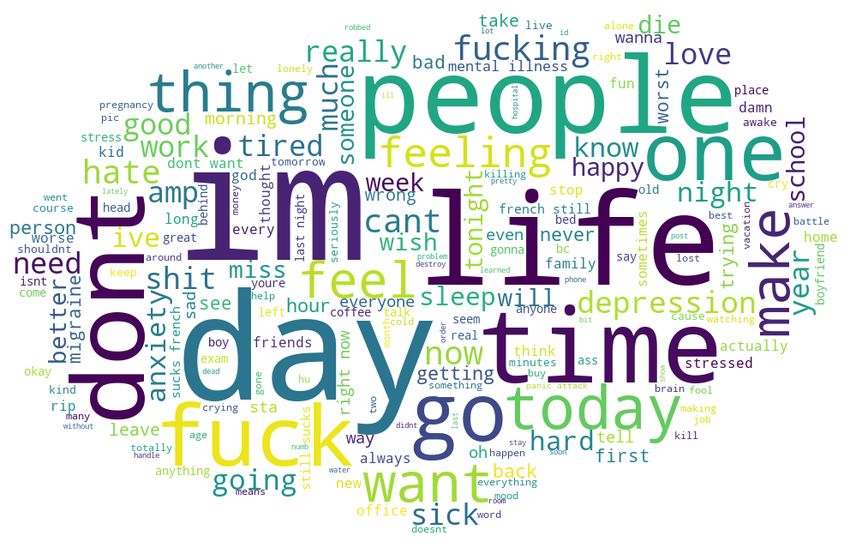
For our standard machine learning models, we represent a Deep learning model specific settings: We use a state of
Tweet by taking the average of the vector of the individual the art deep learning model which is a combination of Con-
words in that Tweet, ignoring the ones that are out of vocab- volutional Neural Network (CNN) layer followed by a Bidi-
ulary. For our deep learning experiments, we take the vector rectional Long Short Term Memory (Bi-LSTM) layer (see
of each word in a Tweet and concatenate them to get a word Figure 4) inspired by the work of (Zhou et al. 2015) and
vector representation of the Tweet. Since this approach will (Nguyen and Nguyen 2017), which we name as cbLSTM.
not create a fixed length word vector representation, we pad
From the train splits (as described in “Train-test splits”
each tweet to make their length equal to the maximum length
section), the deep learning model separates 10% of samples
Tweet in the training set. In the next sections we provide de-
for validation purpose and reports the result on test set. Al-
tailed technical descriptions of our word experimental setup.
though we have the liberty to learn our pre-trained word em-
bedding in our deep learning model, we keep the embed-
Experimental setup ding layer untrainable so that we can report the results that
We experiment with all the 28 combinations from seven fea- reflect only the effectiveness of pre-trained embedding, not
ture extraction methods, such as, BOW, NHEL, LIWC, TE, the learned ones. Moreover, we report results on random ini-
DE, ATE, ATE(orig.) and four standard machine learning tialized embedding to show how the other embeddings im-
models, such as, Multinomial Naı̈ve Bayes (NB), Logistic proved upon it. Since we have a smaller dataset, learning
Regression (LR), Linear Support Vector Machine (LSVM) embedding do not introduce added value.
and Support Vector Machine with radial basis kernel func-
tion (RSVM). In addition, we run experiments on all our 7
http://scikit-learn.org/stable/modules/
four word embeddings and a randomly initialized embed- svm.html
ding representations combined with our deep learning model 8
http://scikit-learn.org/stable/modules/
(cbLSTM) to further analyse the efficacy of our proposed svm.htmlTweets Table 5 and Figure 5.
Category Model-Feat. Prec. Rec. F1
Embedding Layer
Baselines NB-NHEL 0.6338 0.9224 0.7508
LR-BOW 0.6967 0.8264 0.7548
LR-LIWC 0.7409 0.7772 0.7574
RSVM-TE 0.7739 0.7939 0.7824
Dropout = 0.4
Our Models cbLSTM-DE 0.6699 0.8606 0.7526
RSVM-DE 0.7495 0.8280 0.7859
LR-ATE(orig.) 0.7815 0.8020 0.7906
Convolution 1D LSVM-ATE 0.7984 0.8520 0.8239
(Vioulès et al.
Prev. Res. 0.71 0.71 0.71
2018)
Max Pooling 1D
Table 5: Average results on Dataset1 best model-feat combi-
nations
Bi-LSTM (128 Units)
Category Model-Feat. Prec. Rec. F1
Baselines RSVM-NHEL 0.1754 0.7439 0.2858
Dense (64 Units)
RSVM-BOW 0.2374 0.5296 0.3260
RSVM-LIWC 0.2635 0.6750 0.3778
RSVM-TE 0.3485 0.6305 0.4448
Dropout = 0.5 Our Models RSVM-DE 0.3437 0.5198 0.4053
cbLSTM-ATE 0.4416 0.3987 0.4178
RSVM-
0.3476 0.5648 0.4276
ATE(orig.)
Output
RSVM-ATE 0.3675 0.5923 0.4480
(Dense (1 unit)) (Jamil et al.
Prev. Res. 0.1706 0.5939 0.265
2017)
Table 6: Average results on Dataset2 best model-feat combi-
nations
Figure 4: Deep learning model (cbLSTM) architecture
Category Model-Feat. Prec. Rec. F1
Results analysis Baselines
cbLSTM-
0.5464 0.9817 0.6986
Random
Quantitative performance analysis cbLSTM-TE 0.6510 0.8325 0.7262
Here we report the average results (i.e., average Precision, cbLSTM-
Proposed 0.6288 0.8439 0.7093
Recall and F1) for the best performing combinations among ATE(orig.)
all the 28 combinations of our standard machine learning cbLSTM-ATE 0.6915 0.8231 0.7491
cbLSTM-DE 0.6699 0.8606 0.7526
and feature extraction methods (as described in “Experimen-
tal setup” section). We also report the same for our four word Table 7: Average results for deep learning model (cbLSTM)
embeddings combined with the deep learning (cbLSTM) in Dataset1 for all our (Baseline and Proposed) embeddings
model. We report these results separately for our Dataset1
and Dataset2.
Moreover, we report the results of two experiments, one Category Model-Feat. Prec. Rec. F1
by (Vioulès et al. 2018) for Dataset1 and another by (Jamil cbLSTM-
et al. 2017) for Dataset2, where they use their own depres- Baselines 0.2308 0.2791 0.2502
Random
sion lexicons as a feature representation for their machine cbLSTM-TE 0.2615 0.6143 0.3655
learning models. We report these two previous results be- cbLSTM-
Proposed 0.4598 0.3105 0.3671
cause these are the most recent results on depressive Tweets ATE(orig.)
identification task. See Tables 5 and 6. cbLSTM-DE 0.3231 0.4891 0.3880
cbLSTM-ATE 0.4416 0.3987 0.4178
Standard machine learning models: In general, Tweet
level depression detection is a tough problem and a good F1 Table 8: Average results for deep learning model (cbLSTM)
score is hard to achieve (Jamil et al. 2017). Still, our LSVM- in Dataset2 for all our (Baseline and Proposed) embeddings
ATE achieves an average F1 score of 0.8238±0.0259 which
is 4% better than our strongest baseline (RSVM-TE) with In Dataset2, which is imbalanced (90% samples are non-
average F1 score of 0.7824 ± 0.0276 and 11% better than depressive Tweets), our best model RSVM-ATE achieves
(Vioulès et al. 2018) with F1 score of 0.71 in Dataset1, see 0.32% better average F1 score (i.e. 0.4480 ± 0.0209) thanthe strongest baseline, RSVM-TE with average F1 score of
0.4448 ± 0.0197 and 22.3% better F1 score than (Jamil et al.
2017) (i.e. 0.265) , see Table 6 and Figure 6.
In both datasets, NHEL has the best recall and the worst
precision, while, BOW, LIWC and word embedding based
methods have acceptable precision and recall.
Figure 8: Error bars of F1 scores for deep learning models
(cbLSTM) with all our embeddings on Dataset2
F1 score (i.e. 0.7526 ± 0.0244) than the strongest baseline
cbLSTM-TE with average F1 score of 0.7262 ± 0.034. It
slightly performs better (0.35%) than cbLSTM-ATE with
average F1 score of 0.7491 ± 0.0301. In Dataset2, our best
Figure 5: Error bars of F1 scores for our best model-feat. performing model cbLSTM-ATE with average F1 score of
combinations on Dataset1 0.4178 ± 0.0202 performs 5% better than the strongest base-
line cbLSTM-TE with average F1 score of 0.3655 ± 0.021
and around 2% better than close contender cbLSTM-DE
with average F1 score of 0.3880 ± 0.0233, see Figures 7,
8 and Tables 7, 8. However, our best deep learning model
performs on average 5% lower in F1 scores than our stan-
dard machine learning models across our two datasets.
Influence of datasets and feature representations in
predictions
Standard machine learning models: Overall, in both
datasets, word embedding based methods perform much
better than BOW and lexicons. The reason is, they have
a bigger vocabulary and better feature representation than
BOW and lexicons. Among non-word embedding methods,
BOW and LIWC perform better than NHEL, because the
Figure 6: Error bars of F1 scores for our best model-feat. former provide better discriminating features than the latter.
combinations on Dataset2 In Dataset1, ATE achieves better and stable F1 scores than
both TE and DE with DE performing close enough. This
confirms that DE can capture the semantics of depressive
language very well. ATE is superior in performance because
it leverages both the vocabulary coverage and semantics of
a depressive language. In Dataset2, ATE achieves slightly
better (although slightly unstable) F1 score than TE but sig-
nificantly better F1 score than DE. The reason for this could
be that the Tweet samples in Dataset2 are more about gen-
eral distress than actual depression, also dataset is very im-
balanced. In this case, the performance is affected mostly
by the vocabulary size rather than the depressive language
semantics.
Deep learning model: Although the overall F1 scores
Figure 7: Error bars of F1 scores for deep learning models achieved with the deep learning model (cbLSTM) while
(cbLSTM) with all our embeddings on Dataset1 used with the word embeddings is below par than the stan-
dard machine learning models for both datasets, we observe
a general trend of improvement of our proposed ATE and
Deep learning model: In Dataset1, our best performing DE embedding compared to strong baseline TE and random
model cbLSTM-DE achieves around 3% better in average initialized embedding. Moreover this performance improve-ment is more pronounced in our noisy dataset (Dataset2),
unlike standard machine learning models, suggests that deep
learning models might be better at handling noisy data.
Overall, all our proposed embeddings (i.e. DE, ATE) achieve
more stable F1 scores than TE and random embeddings in
both datasets.
We believe the overall under-performance in the deep
learning model is attributed to our small datasets. In our
future analysis of the deep learning models and their per-
formance we intend to experiment with a much larger and
better dataset to derive more insights.
Qualitative performance analysis
We report correctly predicted depressive Tweets in Table 9 Figure 10: Two-dimensional PCA projection of LIWC
by LSVM-ATE (our overall best model) which are mistak- POSEMO and NEGEMO words (frequently occured in our
enly predicted as control Tweets (i.e., false negatives) when datasets) in Adjusted Twitter word Embedding (ATE).
RSVM-TE (our strongest baseline) is used in a test set from
Dataset1. The first example from Table 9, “Tonight may def-
initely be the night”, may be indicative of suicidal ideation According to earlier research, depression has close con-
and should not be taken lightly, also, the second one “0 nection with abnormal regulation of positive and negative
days clean.” is the trade mark indication of continued self- emotion (Kuppens et al. 2012) and (Seabrook et al. 2018).
harm, although many depression detection models will pre- So to consider how the words carrying positive and nega-
dict these as normal Tweets. It is also interesting to see how tive sentiment are situated in our adjusted vector space, we
our best word embedding is helpful in identifying depressive plot the PCA projections of ATE and TE for the high fre-
Tweets which are more subtle like, “Everyone is better off quency words used in both datasets that are the members
without me. Everyone.”. of LIWC positive emotion (POSEMO) and negative emo-
tion (NEGEMO) categories. We observe that POSEMO and
Tweets NEGEMO words form two clearly distinctive clusters, i.e.,
“Tonight may definitely be the night.” C2 and C1 respectively in ATE. We also notice the word
“0 days clean.”
“insomnia” and “sleepless” which represent common sleep
“Everyone is better off without me. Everyone.”
problem in depressed people, reside in C1 or NEGEMO
“Is it so much to ask to have a friend who will be there for
you no matter what?” cluster. However, we do not see any such clusters in TE.
“I understand you’re ‘busy’, but fuck that ... people make See Figure 10 and 9. We believe this distinctions of affective
time for what they want.” contents in vector space partially play a role in our overall
“ I’m a failure.” accuracy. Also the PCA projection gives a glimpse of the
semantic relationship of affective words in depressive lan-
Table 9: False negative depressive Tweets when TE is used, guage. Although its not an exhaustive analysis but a insight-
correctly predicted when ATE is used in a test set from ful one that we believe would be helpful for further analysis
Dataset1. of affect in depressive language.
Effects of embedding augmentation:
The fact that generally ATE performs better (see Tables 5,
6, 7 and 8) than TE proves that our embedding adjustment
improves the semantic representation of TE, because ATE
and TE both have exactly the same vocabulary. Further to
show that embedding adjustment for OOVs contributes to
this improved accuracy, we run an experiment, where we
replace the words in TE which are common to DE, with their
ATE word vectors. We name this embedding, “T E ∩ DE-
in-TE-adjusted.” This confirms that none of the OOVs are
adjusted and we compare this result with our ATE (where
all the OOVs are adjusted). In this experiment, we see T E ∩
DE-in-TE-adjusted obtains 2.62% less F1 score compared
Figure 9: Two-dimensional PCA projection of LIWC to ATE for Dataset1 and 2.13% less F1 score for the same
POSEMO and NEGEMO words (frequently occured in our in Dataset2, confirming semantic adjustment of OOVs does
datasets) in General Twitter word Embedding (TE). play an important role. Also, this model has less stable F1
scores than our best model in both datasets. See Table 10Dataset Model-Feat. F1 Supplementary Results
LR-T E ∩ DE-in-TE-
Dataset1 0.7977 ± 0.0305 Here we report Tables 11, 12, 13 and 14 for the analysis of
adjusted
LSVM-ATE (Best Model) 0.8239 ± 0.0259 our proposed augmentation methods.
RSVM-T E ∩ DE-in-TE-
Dataset2 0.4267 ± 0.0217 Dataset Model-Feat. F1
adjusted
RSVM-ATE (Best Model) 0.4480 ± 0.0209 0.8239 ±
Dataset1 LSVM-ATE (Best Model)
0.0259
RSVM-DE 0.7859 ± 0.0335
Table 10: Average F1 scores from experiments to show the
RSVM-TE 0.7824 ± 0.0276
effect of our augmentation for OOVs RSVM-AT E ∩ DE 0.7786 ± 0.0290
LSVM-T E ∩ DE 0.7593 ± 0.0340
RSVM-T E ∩ DE-concat 0.7834 ± 0.0321
Ethical concerns LR-T E ∩ DE-in-TE-adjusted 0.7977 ± 0.0304
We use Suicidal Forum posts where users are strictly re- 0.4480 ±
Dataset2 RSVM-ATE (Best Model)
quired to stay anonymous. Additionally, it employs active 0.0209
moderators who regularly anonymize the contents in case RSVM-DE 0.4351 ± 0.0206
RSVM-TE 0.4448 ± 0.0196
the user reveals something that can identify them. Moreover,
RSVM-AT E ∩ DE 0.4155 ± 0.028
we use Reddit and Twitter public posts which incur minimal LSVM-T E ∩ DE 0.4002 ± 0.0292
risk of user privacy violation as established by earlier re- RSVM-T E ∩ DE-concat 0.4249 ± 0.0187
search ((Milne et al. 2016), (Coppersmith et al. 2015b) and RSVM-T E ∩ DE-in-TE-adjusted 0.4267 ± 0.0216
(Losada and Crestani 2016)) utilizing the same kind of data.
We also obtained our university ethics board approval that Table 11: Average Precision, Recall and F1 scores from ex-
lets us use datasets collected by external organizations. periments to show the effect of our augmentation
Conclusion
Dataset Model-Feat. F1
In this paper, we empirically present the following observa- Dataset1 LSVM-ATE (Best Model) 0.8239 ± 0.0259
tions for a high quality dataset: LR-ATE-Centroid-1 0.8219 ± 0.0257
• For depressive Tweets detection, we can use word embed- LR-ATE-Centroid-2 0.8116 ± 0.029
ding trained in an unsupervised manner on a small corpus Dataset2 RSVM-ATE (Best Model) 0.4480 ± 0.0209
of depression forum posts, which we call Depression spe- RSVM-ATE-Centroid-1 0.4372 ± 0.0172
RSVM-ATE-Centroid-2 0.4431 ± 0.0211
cific word Embedding (DE), and then use it as a feature
representation for our machine learning models. This ap-
Table 12: Experiments on centroid based methods
proach can achieve good accuracy, despite the fact that it
has 100 times smaller vocabulary than our general Twitter
pre-trained word embedding. Dataset Model-Feat. F1
• Furthermore, we can use DE to adjust the general Twitter Dataset1 LSVM-ATE (Best Model) 0.8239 ± 0.0259
pre-trained word Embedding (available off the shelf) or NB-ATE-AAEME 0.7845 ± 0.0229
TE through non-linear mapping between them. This ad- LR-ATE-AAEME-OOV 0.8014 ± 0.0333
Dataset2 RSVM-ATE (Best Model) 0.4480 ± 0.0209
justed Twitter word Embedding (ATE) helps us achieve
RSVM-ATE-AAEME 0.4166 ± 0.0187
even better results for our task. RSVM-ATE-AAEME-OOV 0.4433 ± 0.0200
• We need not to depend on human annotated data or la-
belled data for any of our word embedding representation Table 13: Experiments on meta-embedding methods
creation.
• Depression forum posts have specific distributed repre- Dataset Model-Feat. F1
sentation of words and it is different than that of general 0.8239 ±
twitter posts and this is reflected in ATE, see Figure 10. Auto-Encoder Based Methods ATE (Best Model)
0.0259
• We intend to make our depression corpus and embeddings ATE-AAEME 0.7845 ± 0.0229
publicly available upon acceptance of our paper. ATE-AAEME-OOV 0.8014 ± 0.0333
Centroid Based Methods ATE-Centroid-1 0.8219 ± 0.0257
ATE-Centroid-2 0.8116 ± 0.029
Future work
In the future, we would like to analyze DE more exhaus- Table 14: Experiments on meta-embedding and centroid
tively to find any patterns in semantic clusters that specif- based methods on Dataset-1
ically identify depressive language. We would also like to
use ATE for Twitter depression lexicon induction and for
discovering depressive Tweets. We can see great promise in References
its use in creating a semi-supervised learning based auto- [Asgari and Mofrad 2015] Asgari, E., and Mofrad, M. R.
mated depression data annotation task later on. 2015. Continuous distributed representation of biologicalsequences for deep proteomics and genomics. PloS one cial media text. In Eighth International Conference 10(11):e0141287. on Weblogs and Social Media (ICWSM-14). Available at [Bengio and Heigold 2014] Bengio, S., and Heigold, G. (20/04/16) http://comp. social. gatech. edu/papers/icwsm14. 2014. Word embeddings for speech recognition. In Fifteenth vader. hutto. pdf. Annual Conference of the International Speech Communica- [Godin et al. 2015] Godin, F.; Vandersmissen, B.; De Neve, tion Association. W.; and Van de Walle, R. 2015. Multimedia lab @ acl wnut [Bollegala and Bao 2018] Bollegala, D., and Bao, C. 2018. ner shared task: Named entity recognition for twitter micro- Learning word meta-embeddings by autoencoding. In Pro- posts using distributed word representations. In Proceedings ceedings of the 27th International Conference on Computa- of the Workshop on Noisy User-generated Text, 146–153. tional Linguistics, 1650–1661. [Greenberg et al. 2015] Greenberg, P. E.; Fournier, A.-A.; [Boyd et al. 1982] Boyd, J. H.; Weissman, M. M.; Thomp- Sisitsky, T.; Pike, C. T.; and Kessler, R. C. 2015. The eco- son, W. D.; and Myers, J. K. 1982. Screening for de- nomic burden of adults with major depressive disorder in pression in a community sample: Understanding the discrep- the united states (2005 and 2010). The Journal of clinical ancies between depression symptom and diagnostic scales. psychiatry 76(2):155–162. Archives of general psychiatry 39(10):1195–1200. [Jamil et al. 2017] Jamil, Z.; Inkpen, D.; Buddhitha, P.; and [Cheng et al. 2016] Cheng, P. G. F.; Ramos, R. M.; Bitsch, White, K. 2017. Monitoring tweets for depression to de- J. Á.; Jonas, S. M.; Ix, T.; See, P. L. Q.; and Wehrle, K. 2016. tect at-risk users. In Proceedings of the Fourth Workshop on Psychologist in a pocket: lexicon development and content Computational Linguistics and Clinical Psychology—From validation of a mobile-based app for depression screening. Linguistic Signal to Clinical Reality, 32–40. JMIR mHealth and uHealth 4(3). [Kiritchenko, Zhu, and Mohammad 2014] Kiritchenko, S.; [Coppersmith et al. 2015a] Coppersmith, G.; Dredze, M.; Zhu, X.; and Mohammad, S. M. 2014. Sentiment analysis Harman, C.; Hollingshead, K.; and Mitchell, M. 2015a. of short informal texts. Journal of Artificial Intelligence Clpsych 2015 shared task: Depression and ptsd on twitter. Research 50:723–762. In Proceedings of the 2nd Workshop on Computational Lin- [Kuppens et al. 2012] Kuppens, P.; Sheeber, L. B.; Yap, guistics and Clinical Psychology: From Linguistic Signal to M. B.; Whittle, S.; Simmons, J. G.; and Allen, N. B. 2012. Clinical Reality, 31–39. Emotional inertia prospectively predicts the onset of depres- [Coppersmith et al. 2015b] Coppersmith, G.; Dredze, M.; sive disorder in adolescence. Emotion 12(2):283. Harman, C.; and Hollingshead, K. 2015b. From adhd to sad: [Losada and Crestani 2016] Losada, D. E., and Crestani, F. Analyzing the language of mental health on twitter through 2016. A test collection for research on depression and self-reported diagnoses. In Proceedings of the 2nd Work- language use. In International Conference of the Cross- shop on Computational Linguistics and Clinical Psychol- Language Evaluation Forum for European Languages, 28– ogy: From Linguistic Signal to Clinical Reality, 1–10. 39. Springer. [Coppersmith, Dredze, and Harman 2014] Coppersmith, G.; [Mikolov et al. 2013a] Mikolov, T.; Sutskever, I.; Chen, K.; Dredze, M.; and Harman, C. 2014. Quantifying mental Corrado, G. S.; and Dean, J. 2013a. Distributed represen- health signals in twitter. In Proceedings of the Workshop on tations of words and phrases and their compositionality. In Computational Linguistics and Clinical Psychology: From Advances in neural information processing systems, 3111– Linguistic Signal to Clinical Reality, 51–60. 3119. [De Choudhury and De 2014] De Choudhury, M., and De, S. [Mikolov et al. 2013c] Mikolov, T.; Chen, K.; Corrado, G.; 2014. Mental health discourse on reddit: Self-disclosure, and Dean, J. 2013c. Efficient estimation of word represen- social support, and anonymity. In ICWSM. tations in vector space. arXiv preprint arXiv:1301.3781. [De Choudhury et al. 2013b] De Choudhury, M.; Gamon, [Mikolov, Le, and Sutskever 2013b] Mikolov, T.; Le, Q. V.; M.; Counts, S.; and Horvitz, E. 2013b. Predicting depression and Sutskever, I. 2013b. Exploiting similarities via social media. In ICWSM, 2. among languages for machine translation. arXiv preprint [De Choudhury 2013a] De Choudhury, M. 2013a. Role of arXiv:1309.4168. social media in tackling challenges in mental health. In [Miller 1995] Miller, G. A. 1995. Wordnet: a lexi- Proceedings of the 2nd international workshop on Socially- cal database for english. Communications of the ACM aware multimedia, 49–52. ACM. 38(11):39–41. [Dodds et al. 2011] Dodds, P. S.; Harris, K. D.; Kloumann, [Milne et al. 2016] Milne, D. N.; Pink, G.; Hachey, B.; and I. M.; Bliss, C. A.; and Danforth, C. M. 2011. Temporal Calvo, R. A. 2016. Clpsych 2016 shared task: Triaging patterns of happiness and information in a global social net- content in online peer-support forums. In Proceedings of the work: Hedonometrics and twitter. PloS one 6(12):e26752. Third Workshop on Computational Lingusitics and Clinical [Faruqui et al. 2015] Faruqui, M.; Dodge, J.; Jauhar, S. K.; Psychology, 118–127. Dyer, C.; Hovy, E.; and Smith, N. A. 2015. Retrofitting word [Mohammad and Kiritchenko 2015] Mohammad, S. M., and vectors to semantic lexicons. In Proceedings of NAACL. Kiritchenko, S. 2015. Using hashtags to capture fine emo- [Gilbert 2014] Gilbert, C. H. E. 2014. Vader: A parsi- tion categories from tweets. Computational Intelligence monious rule-based model for sentiment analysis of so- 31(2):301–326.
You can also read