A hierarchical knowledge-based classification for glacier terrain mapping: a case study from Kolahoi Glacier, Kashmir Himalaya - Cambridge ...
←
→
Page content transcription
If your browser does not render page correctly, please read the page content below
Annals of Glaciology 57(71) 2016 doi: 10.3189/2016AoG71A046                                                                                              1
       © The Author(s) 2016. This is an Open Access article, distributed under the terms of the Creative Commons Attribution licence (http://creativecommons.
       org/licenses/by/4.0/), which permits unrestricted re-use, distribution, and reproduction in any medium, provided the original work is properly cited.

         A hierarchical knowledge-based classification for glacier terrain
         mapping: a case study from Kolahoi Glacier, Kashmir Himalaya
                                                                Aparna SHUKLA,1 Iram ALI2
                                                1
                                                 Wadia Institute of Himalayan Geology (WIHG), Dehradun, India
                                            2
                                                Department of Earth Sciences, University of Kashmir, Srinagar, India
                                                 Correspondence: Aparna Shukla

                    ABSTRACT. A glacierized terrain comprises different land covers, and their mapping using satellite
                    data is challenged by their spectral similarity. We propose a hierarchical knowledge-based classification
                    (HKBC) approach for differentiation of glacier terrain classes and mapping of glacier boundaries, using
                    Advanced Spaceborne Thermal Emission and Reflection Radiometer (ASTER) imagery and Global
                    Digital Elevation Model (GDEM). The methodology was tested over Kolahoi Glacier, Kashmir Himalaya.
                    For the sequential extraction of various glacier terrain classes, several input layers were generated from
                    the primary datasets by applying image-processing techniques. Noticeable differences in temperature
                    and spectral response between supraglacial debris and periglacial debris facilitated the development of
                    a thermal glacier mask and normalized-difference debris index, which together with slope enabled their
                    differentiation. These and the other layers were then used in several discrete tests in HKBC, to map
                    various glacier terrain classes. An ASTER visible near-infrared image and 42 field points were used to
                    validate results. The proposed approach satisfactorily classified all the glacier terrain classes with an
                    overall accuracy of 89%. The Z-test reveals that results obtained from HKBC are significantly (at 95%
                    confidence level) better than those from a maximum likelihood classifier (MLC). Glacier boundaries
                    obtained from HKBC were found to be plausibly better than those obtained from MLC and
                    visual interpretation.
                    KEYWORDS: debris-covered glaciers, glacier delineation, glacier mapping, supraglacial debris

       INTRODUCTION                                                                            (Keshri and others, 2009; Burns and Nolin, 2014; Bhardwaj
       As an integral part of the cryosphere, mountain glaciers                                and others, 2015); (3) morphometric analysis of attributes
       constitute one of the most important components of the                                  such as slope, aspect and elevation (Bolch and others, 2007;
       Earth’s natural system and serve as sensitive climate-change                            Shukla and others, 2010a); (4) multi-source and texture
       indicators (Scherler and others, 2011). Therefore, their                                analysis (Paul and others, 2004; Racoviteanu and Williams,
       accurate mapping and monitoring are of vital importance                                 2012); and (5) supervised classification (Bayr and others,
       for the proper planning and management of water resources.                              1994; Shukla and others, 2009; Khan and others, 2015).
       Considering the extent and inaccessibility of glaciers,                                 These research methodologies have mapped glacier facies
       remote sensing acts as an effective technology for their                                with varying success and have been effective in distinguish-
       regular mapping in a comprehensive and effective manner                                 ing debris-free glacier ice from debris cover, but report
       (Bolch and others, 2010; Bhambri and others, 2011; Paul                                 difficulties in separating debris on the glacier surface from
       and Mölg, 2014). Precise areal extents of various glacier                               surrounding terrain (Shukla and others, 2010a,b; Raco-
       terrain classes are directly or indirectly used in various                              viteanu and Williams, 2012). Debris may be present either
       studies. Different snow-ice classes (e.g. dry snow, wet snow,                           on the surface of the glacier, called supraglacial debris
       ice, ice-mixed debris) have different water storage capacity,                           (SGD), or along the margins of the glacier, called periglacial
       and changes or inter-conversions between them greatly                                   debris (PGD) (Shukla and others, 2010a). In the ablation
       influence the storage of glaciers (Jansson and others, 2003).                           zone, towards the glacier terminus, as ice starts giving way
       Dry and wet snow areas are important for avalanche                                      to supraglacial debris, there forms a mixture of the two
       vulnerability assessment. Differentiation of snow and ice                               classes called ice-mixed debris (IMD) (Keshri and others,
       also facilitates mass-balance estimates based on obser-                                 2009), also sometimes referred to as ‘dirty glacier ice’ or
       vations of the accumulation–area ratio. Thus, accurate                                  ‘mixed ice’ (Bhardwaj and others, 2015). This mixed class
       mapping of these classes would greatly influence the                                    covers a region between the total ice-covered area in the
       precision of hydrological modelling, avalanche prediction/                              upper reaches of the ablation zone and the total debris-
       forecasting models and glacier mass-balance studies. Also,                              covered area in the lower reaches of the ablation zone, i.e.
       correct quantification of the areal extents of the supraglacial                         the glacier snout. Both SGD and PGD originate from
       debris and its temporal variations may give a clear                                     surrounding valley rock, and are indistinguishable on
       indication of the glacier’s health (Shukla and others, 2009;                            multispectral satellite images. Thus, they act as a major
       Racoviteanu and Williams, 2012; Reid and Brock, 2014).                                  constraint on accurate satellite-based mapping of glaciers
          Techniques for glacier-cover mapping include (1) band                                (Paul and others, 2004, 2013; Shukla and others, 2010a).
       ratio techniques (Kääb, 2002; Paul and others, 2013);                                   Differentiation of SGD and PGD classes can facilitate
       (2) image classification techniques based on spectral indices                           automatic glacier mapping (Shukla and others, 2010a,b).

Downloaded from https://www.cambridge.org/core. 25 Aug 2021 at 18:13:58, subject to the Cambridge Core terms of use.
2 Shukla and Ali: HKBC for glacier terrain mapping
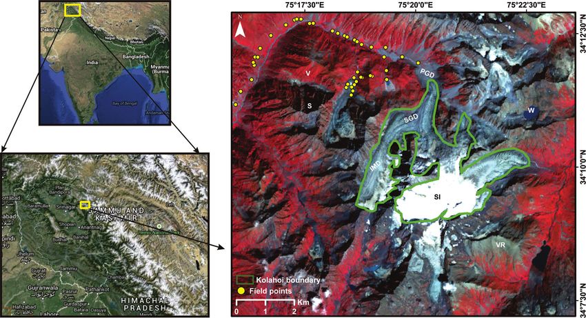
Fig. 1. The ASTER false-colour composite on the right shows Kolahoi Glacier and the adjoining area, with band combination R = near
infrared, G = red and B = green band. In this map the abbreviations are W: water; V: vegetation; SI: snow-ice; S: shadow; IMD: ice-mixed
debris; SGD: supraglacial debris; PGD: periglacial debris; VR: valley rock. Circles represent the set of field-based observations collected
during September 2014. Zoomed-out images on left show location of the study site within the region (bottom) and of the region within the
subcontinent (top).
Many works have reported this problem and have proposed STUDY AREA
improved techniques for mapping the margins of glaciers The current study is focused on Kolahoi Glacier and the
with varying amounts of debris cover in the ablation area. adjoining areas (34°110 –34°210 N, 75°270 –75°390 E), located
A literature review suggests that optical data alone are in Lidder valley, western Himalaya (Fig. 1). The meltwater
insufficient for mapping glacier margins, especially when stream of Kolahoi Glacier is known as the West Lidder River
they are covered with varying amounts of debris. Previous and joins the East Lidder River at Pahalgam (35 km from the
studies have shown that inputs from other sources such as snout). Pahalgam is connected to Srinagar by road and from
geomorphometry (Bolch and Kamp, 2006), thermal data there to Aru (i.e. first 11 km). Beyond that, the remaining
(Ranzi and others, 2004) or a combination of these (Paul and 24 km to the glacier snout have to be covered either on foot
others, 2004; Bolch and other, 2008; Shukla and others, or by pony (Ahmad and Hashmi, 1974). The glacier is �5 km
2010a,b; Bhambri and others, 2012; Karimi and others, long and has an area of �11 km2. Its headwall is located at
2012; Tiwari and others, in press) are needed together with 5425 m a.s.l. on Kolahoi mountain, between the peaks of
optical data for effective mapping of glacier margins. Dudnag in the west and Hiurbagwan in the east (Kaul, 1990).
Recently Bhardwaj and others (2015) demonstrated a Land- The glacier surface is marked by crevasses along the eastern
sat 8 Operational Land Imager sensor based algorithm for margins of the ablation zone and an extensive mass of debris
automated mapping of glacier facies and supraglacial debris. along the western margin (Kaul, 1990).
This method used a manually digitized glacier boundary for Records of previous visits to, and studies on, Kolahoi
extracting the glacier area to map glacier facies within it, and Glacier suggest that the focus was mainly on field mapping
does not consider separation of SGD from surrounding (Neve, 1910), estimates of retreat (Neve, 1910; Odell, 1963;
terrain. However, most of these studies either have ambitious Kaul, 1990; Kanth and others, 2011), geomorphology and
data and processing requirements, complex procedural steps palaeoglaciation (Ahmad and Hashimi, 1974; Kaul, 1990) of
or have transferability issues (Tiwari and others, in press), the glacier. However, to date, there has been no study
which limits repeated applicability. reported on differentiation of glacier facies and boundary
Thus, there is still a need to devise a methodology that mapping of Kolahoi Glacier.
may prove more efficient and consistent in mapping various
glacier terrain classes (snow-ice, vegetation, water, IMD,
SGD, PGD and valley rock), leading towards automatic DATA AND METHODOLOGY
mapping of glacier boundaries. To this end, a hierarchical
knowledge-based approach is proposed here for sequential Dataset used
differentiation of various glacier terrain classes, with Advanced Spaceborne Thermal Emission and Reflection
particular emphasis on SGD, PGD and valley rock owing Radiometer (ASTER) data acquired on 20 September 2003
to their spectral similarity. were selected as the primary dataset, on the basis of minimal
Downloaded from https://www.cambridge.org/core. 25 Aug 2021 at 18:13:58, subject to the Cambridge Core terms of use.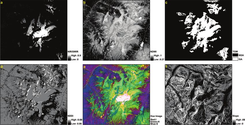
Shukla and Ali: HKBC for glacier terrain mapping                                                                                                          3

       Table 1. Description of the spectral indices discussed in this study. Formulation subscripts indicate ASTER band numbers

       Spectral index                             Source                                   Formulation                                    Utility

                                                                                    Greenðast b1Þ SWIRðast b5Þ
       Normalized-difference                 Dozier (1989)                    NDSI ¼                                   Mapping and differentiating between snow-ice
                                                                                    Greenðast b1Þ þ SWIRðast b5Þ
       snow index (NDSI)                                                                                                covered areas and non-snow-and-ice areas
                                                                                    SWIRðast b6Þ     TIRðast b14Þ
       Normalized-difference                    This study                   NDDI ¼                                     Mapping and differentiating between supra-
                                                                                     SWIRðast b6Þ þ TIRðast b14Þ
       debris index (NDDI)                                                                                                 glacial debris and that of the terrain
                                                                                    Greenðast b1Þ     NIRðast b3Þ
       Normalized-difference                McFeeters (1996)                 NDWI ¼                                               Mapping surface water
                                                                                     Greenðast b1Þ þ NIRðast b3Þ
       water index (NDWI)                                                           Greenðast b1Þ     Redðast b2Þ
       Normalized-difference           Keshri and others (2009)              NDGI ¼                                    Mapping and differentiating between snow-ice
                                                                                     Greenðast b1Þ þ Redðast b2Þ
       glacier index (NDGI)                                                                                                    and ice-mixed debris class

       cloud cover, good contrast between various land covers and                              nearest-neighbour interpolation in order to match the spatial
       suitable acquisition date (ablation season). The scene was                              resolution of the visible bands for band ratio computations.
       devoid of seasonal snow cover. Two ASTER data products,
       namely AST14DMO (registered at sensor L1B) and AST08                                    Derivation of the knowledge base
       (surface kinetic temperature), were downloaded free of                                  The approach proposed here requires several input layers:
       charge from NASA’s Earth Observing System Data and                                      NIR/SWIR ratio and spectral indices (normalized-difference
       Information System (https://reverb.echo.nasa.gov), under the                            glacier index (NDGI), normalized-difference water index
       auspices of the Global Land Ice Measurements from Space                                 (NDWI), normalized-difference debris index (NDDI))
       (GLIMS) project. The ASTER Global Digital Elevation Model                               (Table 1), image transformations (intensity hue saturation
       (ASTER GDEM v2), which is freely available, was also                                    (IHS) image), topographic attributes (slope) and the thermal
       downloaded from the US Geological Survey (USGS) website                                 glacier mask (TGM). The various processing steps involved
       (http://glovis.usgs.gov/). Additionally, 42 field-based obser-                          in generating these input layers are discussed next.
       vations were collected during September 2014, using a                                      The NIR/SWIR ratio image (Fig. 2a) and NDGI (Keshri and
       handheld Trimble GPS (Fig. 1). Such GPS devices provide                                 others, 2009) were obtained from multispectral ASTER data
       horizontal accuracy of up to �3.9 m and vertical accuracy                               for mapping of snow-ice and IMD. The normalized-differ-
       of �15 m in mountainous terrain (Racoviteanu and others,                                ence snow index (NDSI) was also tested, but not used here as
       2007; Bhardwaj and others, 2015). The comparison of                                     it misclassified water bodies as snow-ice, probably because
       z-coordinates of the field points and corresponding elev-                               of their similar bulk optical properties in the VNIR (Dozier,
       ations of the GDEM showed a mean difference and standard                                1989). The NDWI (Fig. 2b) was derived from ASTER1 and
       deviation of –33 m and 23 m, which we take as the offset                                ASTER3 bands and facilitated the delineation of water
       and uncertainty, respectively. Information regarding the                                (McFeeters, 1996). Many previous studies have applied
       glacier terrain classes (vegetation, water, PGD, SGD and                                band ratio algorithms for mapping of snow-ice, IMD and
       valley rock) present at these measurement points was                                    water, with satisfactory results (Paul and others, 2004; Bolch
       recorded and later used to assess the positional accuracy                               and Kamp, 2006; Keshri and others, 2009; Racoviteanu and
       of the glacier terrain classes mapped using hierarchical                                Williams, 2012).
       knowledge-based classification (HKBC).                                                     Nevertheless, the main challenge in the current study was
                                                                                               to differentiate and map PGD and SGD. To achieve their
       Implementation of HKBC                                                                  differentiation, two new input layers (TGM and NDDI) were
       Mapping of various glacier terrain classes (snow-ice,                                   generated which depend upon the optical and thermal
       vegetation, water, IMD, SGD, PGD and valley rock) using                                 characteristics of these classes (Fig. 3a and b). Past remote-
       HKBC involves several steps, namely data preprocessing,                                 sensing studies have revealed that there exists considerable
       derivation of the knowledge base and hierarchical classifi-                             temperature difference between SGD and PGD cover classes
       cation of glacier terrain classes, which are described below.                           (Taschner and Ranzi, 2002; Ranzi and others, 2004; Shukla
                                                                                               and others, 2010a), probably due to glacial ice present
       Preprocessing of data                                                                   beneath the SGD. This has been used by some workers as a
       Preprocessing involved the conversion of visible near-                                  source of additional information for segregation of PGD and
       infrared (VNIR) and shortwave infrared (SWIR) data to                                   SGD (Shukla and others, 2010a; Casey and others, 2012).
       reflectance, and thermal data to brightness temperature.                                Using this preliminary idea, an in-depth investigation of
       Optical data were first converted to radiance, then radio-                              surface temperatures was carried out and it was observed
       metric (atmospheric and topographic) corrections were                                   that the surface temperature of glacier cover classes (snow-
       applied to retrieve reflectance values. Details of these                                ice, IMD and SGD) does not exceed 283 K. Therefore, this
       procedures are provided by Shukla and others (2010a). It is                             criterion has been applied here for generation of a TGM,
       pertinent to mention that coefficients of determination                                 separating the classes with temperature below 283 K as
       obtained by regression between corrected reflectance and                                glacier cover classes (snow-ice, IMD and SGD), from the
       terrain illumination were found to be near zero (r2 = �0.005),                          classes with temperature above 283 K as non-glacier cover
       suggesting minimal effect of topography. Atmospherically                                classes (PGD, vegetation, water and valley rock) (Fig. 2c).
       corrected radiances of thermal infrared (TIR) bands were                                The TGM so obtained is a binary map (TGM = 0 for non-
       converted to brightness temperatures (K) using Planck’s                                 glacier area and TGM = 1 for glacier area; Fig. 2c). The
       radiation equation (Yin and others, 2013). Finally, ASTER                               temperatures of the non-glacier cover classes in the
       SWIR, thermal bands and GDEM were resampled to 15 m by                                  shadowed regions were found to exceed those of glacier

Downloaded from https://www.cambridge.org/core. 25 Aug 2021 at 18:13:58, subject to the Cambridge Core terms of use.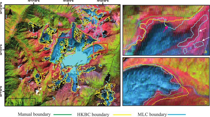
4                                                                                                           Shukla and Ali: HKBC for glacier terrain mapping

           Fig. 2. The main input layers used in the hierarchical knowledge-based classifier: (a) NIR/SWIR (values 0–0.9); (b) normalized difference
           water index (values 0.27–1); (c); thermal glacier mask (TGM) (NGA: non-glacier area, GA: glacier area); (d) normalized-difference debris
           index (NDDI) (values 0.06–0.68); (e) hue image (values 0.074–1); and (f) slope map (values 0–89).

           cover classes. This is in agreement with the results obtained                           due to the underlying glacier ice. The contrasting spectral
           by Shukla and others (2010b) and Karimi and others (2012).                              response of these classes was used to formulate a new index,
              Observing the spectral curves of SGD vis-à-vis other                                 the NDDI. The SWIR and TIR bands were normalized before
           classes, it was noticed that SGD showed higher response in                              creation of NDDI in order to resolve the dimensional
           the SWIR region (ASTER band 6), similar to PGD and valley                               conflict. This index highlights the supraglacial debris in the
           rock (Fig. 3a and b), because the three are compositionally                             region (Fig. 2d). The formulation of the index is given in
           the same. However, the response of supraglacial debris                                  Table 1. Thus, both TGM and NDDI were employed to
           deviates considerably from the other two classes (PGD and                               separate SGD from PGD and valley rock.
           valley rock) in the TIR region (ASTER band 14). This is                                    ASTER bands 1–3 were transformed to intensity–hue–
           because SGD has lower temperature than PGD and valley                                   saturation (IHS) space (Fig. 2e). The hue component high-
           rock (Taschner and Ranzi, 2002; Ranzi and others, 2004)                                 lighted the vegetated area (purple) and thus facilitated the

           Fig. 3. (a) Spectral response curves derived from ASTER image; (b) zoomed-in view of spectral response curve from B6 to B14. Coloured
           lines represent the spectral behaviour of various classes. The x-axis represents different ASTER spectral bands (B1–B14). The y-axis denotes
           percentage spectral radiance. PGD: periglacial debris; SGD: supraglacial debris; IMD: ice-mixed debris.

Downloaded from https://www.cambridge.org/core. 25 Aug 2021 at 18:13:58, subject to the Cambridge Core terms of use.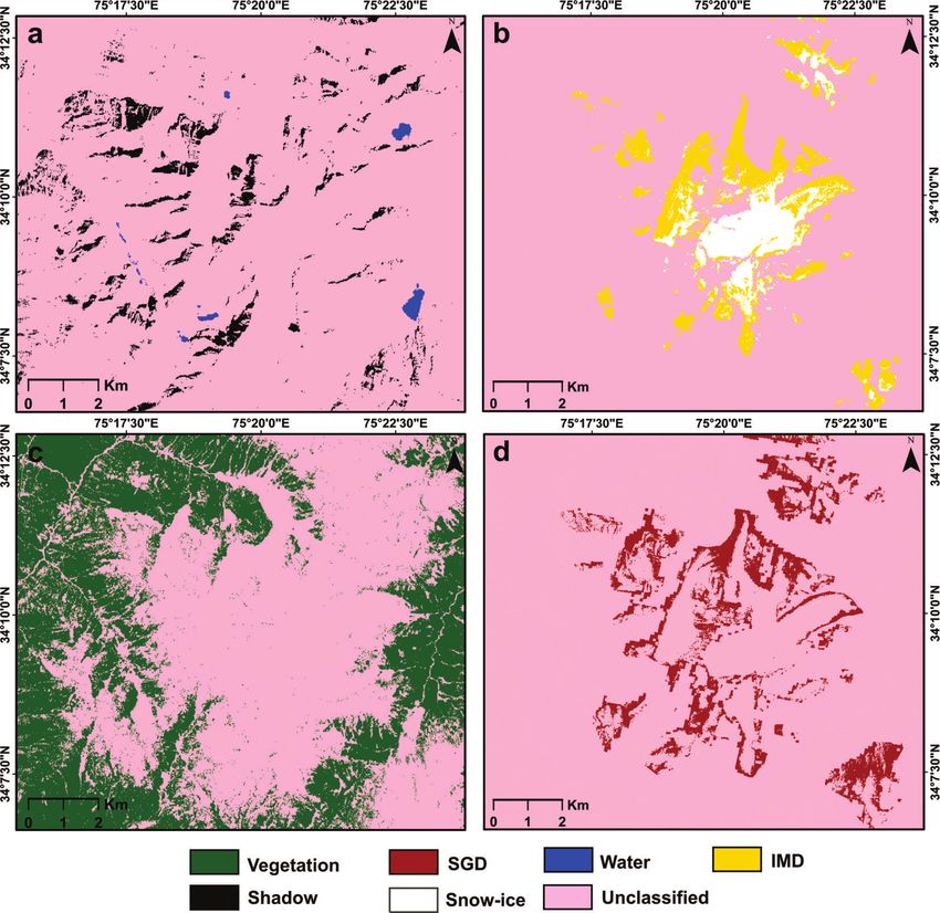
Shukla and Ali: HKBC for glacier terrain mapping                                                                                                      5

       Fig. 4. Conceptual flow chart of the HKBC scheme for glacier terrain mapping. TH: threshold; NDWI: normalized-difference water index;
       NDGI: normalized-difference glacier index; IHS: intensity hue saturation; TGM: thermal glacier mask; NDDI: normalized-difference debris
       index; IMD: ice-mixed debris; SGD: supraglacial debris. Final Map constitutes shadow, water, snow-ice, IMD, vegetation, SGD, periglacial
       debris and valley rock.

       extraction of vegetation (Fig. 2e). Paul and others (2004) and                          threshold as it is known that sparse vegetation can grow on
       Racoviteanu and Williams (2012) have previously used the                                debris-covered parts of glaciers during spring (Bolch and
       IHS transformation to map vegetation and bare rock. A slope                             others, 2007).
       map (Fig. 2f) derived from the ASTER GDEM facilitated the                                   (d) Supraglacial debris
       separation of PGD and valley rock. DEM-derived attributes                                   TGM and NDDI were used to map the SGD in the area,
       (slope, aspect and curvature) have been used for glacier                                by employing a threshold of 0.115 (TGM = 1 or NDDI >
       terrain mapping in previous studies (Paul and others, 2004;                             0.115 = SGD) (Figs 4 and 5d). TGM was able to classify
       Bolch and others, 2010; Racoviteanu and Williams, 2012).                                those regions as SGD where NDDI could not map it and
                                                                                               vice versa.
       Hierarchical classification of glacier terrain classes                                      (e) Periglacial debris and valley rock
       Under this heading, we describe the individual steps                                        In-depth analysis of the slope values showed that the
       followed in HKBC for mapping different glacier terrain                                  debris-covered regions had a slope range of 0–24°. A
       classes. The processing workflow is schematically shown in                              maximum value of 24° (slope < 24° = PGD, else valley rock)
       Figure 4.                                                                               was selected to map PGD in agreement with previous
          (a) Shadow and water                                                                 studies (Paul and others, 2004; Karimi and others, 2012),
          Before mapping any glacier terrain class, the shadowed                               which suggest that most of the debris-covered regions can
       regions were automatically delineated using ASTER band 3,                               be captured at this slope threshold since debris tends to rest
       and a threshold value of 0.043 (band 3 < 0.043 = shadow)                                on gentler slopes (Fig. 4). This step resulted in the final
       was applied (Fig. 4). This helped to reduce misclassifications                          glacier terrain map, showing PGD (grey) and valley rock
       among glacier terrain classes. Racoviteanu and Williams                                 (tan) in addition to the other glacier terrain classes discussed
       (2012) adopted a similar approach to remove shadowed                                    above (Fig. 6a).
       regions. In the same step, water was differentiated by                                      Once the glacier terrain classes have been mapped, the
       NDWI, applying a threshold of 0.35 (NDWI < 0.35 = water).                               glacier boundary can be delineated by merging the glacier
       The shadowed areas are shown in black, and water as blue,                               cover (i.e. snow-ice, IMD and SGD) and non-glacier cover
       in Figure 5a.                                                                           (i.e. PGD, valley rock, water, shadow and vegetation)
          (b) Snow-ice and IMD                                                                 classes (Shukla and others, 2010a).
          Both snow-ice and IMD were mapped using the NIR/
       SWIR ratio image and NDGI. A threshold value of 0.45
       (NIR/SWIR > 0.45 = snow-ice) was found to be suitable for                               RESULTS AND DISCUSSION
       snow-ice, and for IMD a threshold of 0.4 (NDGI < 0.4 =                                  The efficiency of the proposed HKBC approach for mapping
       IMD) was found to be satisfactory (Figs 4 and 5b). Snow was                             various glacier terrain classes was tested by a two-way
       more prevalent than ice, but the classification does not                                accuracy assessment process. First, the accuracy of the
       distinguish between them.                                                               glacier terrain maps obtained via HKBC and MLC was
          (c) Vegetation                                                                       assessed against the reference image (ASTER VNIR).
          The hue and NIR/SWIR images were found to be useful                                  Secondly, the boundary of the glacier delineated using the
       for mapping vegetation with a threshold of 0.48 and 0.45,                               glacier terrain map was evaluated against the manually
       respectively (Hue > 0.48 and NIR/SWIR > 0.45 = vegetation)                              digitized boundary of the glacier (by visual interpretation of
       (Figs 4 and 5c). Caution was exercised in selecting this                                the ASTER VNIR image).

Downloaded from https://www.cambridge.org/core. 25 Aug 2021 at 18:13:58, subject to the Cambridge Core terms of use.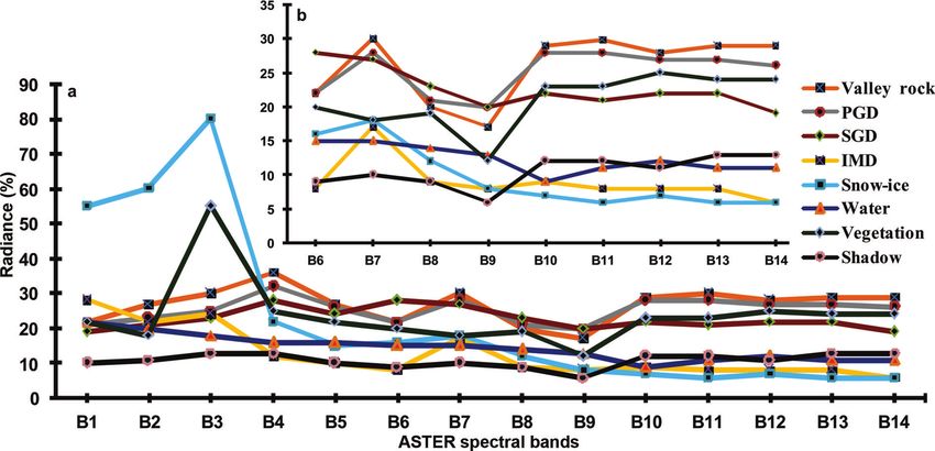
6                                                                                                           Shukla and Ali: HKBC for glacier terrain mapping

           Fig. 5. Six of the classes obtained through HKBC: (a) shadowed areas in black, and water in blue; (b) snow-ice in white, and gold pertaining
           to ice-mixed debris; (c) vegetation in green; (d) SGD in brown. SGD: supraglacial debris; IMD: ice-mixed debris.

           Accuracy of glacier terrain mapping                                                     no higher-resolution image available for this date. To
           The final glacier terrain map obtained from HKBC was                                    determine the efficacy of HKBC, conventional-error-matrix
           validated against the ASTER VNIR image (15 m spatial                                    based measures, namely overall user’s and producer’s
           resolution) and 42 field-based observations. The ASTER                                  accuracy (Foody, 2002), were determined (Table 2). The
           VNIR image was considered as reference because there was                                overall accuracy (OA) is used to indicate the accuracy of the
                                                                                                   whole classification (i.e. number of correctly classified pixels
                                                                                                   divided by total number of testing pixels). OA does not take
                                                                                                   into account the off-diagonal elements of the error matrix
           Table 2. User’s accuracy (UA) and producer’s accuracy (PA) of                           which represent the misclassification errors, i.e. errors of
           individual glacier terrain classes derived from HKBC and maximum                        omission and commission. However, the kappa coefficient
           likelihood classifier (MLC). The overall accuracy produced by
                                                                                                   does take these errors into account, and is thus considered a
           HKBC is 89%, and a kappa coefficient of 0.86 and MLC resulted in
           an overall accuracy of 63% with a kappa coefficient of 0.60
                                                                                                   better estimate of classification accuracy. Corresponding to
                                                                                                   these errors, a new set of accuracy measures may be derived:
                                                                                                   producer’s accuracy (PA) and user’s accuracy (UA). The PA
           Class name                   HKBC                              MLC
                                                                                                   relates to the probability that a reference sample is correctly
                                 UA%             PA%             UA%              PA%              mapped and measures the error of omission. The UA
                                                                                                   indicates the probability that a sample from the classified
           Snow-ice               91              94               89              83              map actually matches what it is in the reference data and
           IMD                    91              85               62              70              measures the commission error. High individual accuracies
           SGD                    81              88               41              46              with minimal difference between them indicate accurate
           PGD                    78              81               36              35
                                                                                                   differentiation of the concerned class.
           Valley rock            87              80               49              45
           Vegetation             95              100              91              92
                                                                                                      A testing dataset constituting 650 pixels was taken using
           Water                  88              93               69              85              stratified random sampling, and additionally 42 ground
           Shadow                 89              83               53              48              control points (692 points in total) were taken for evaluating
                                                                                                   the accuracy of various glacier terrain classes. Reference

Downloaded from https://www.cambridge.org/core. 25 Aug 2021 at 18:13:58, subject to the Cambridge Core terms of use.
Shukla and Ali: HKBC for glacier terrain mapping 7
Fig. 6. Comparison of the glacier terrain mapping from the proposed HKBC and supervised classification (MLC). (a) Final map obtained from
HKBC scheme; (b) map obtained from MLC. The rectangles in (a) and (b) are enlarged in (c) and (d) respectively. SGD: supraglacial debris;
IMD: ice-mixed debris; PGD: periglacial debris.
classes for all the testing pixels were derived on the basis of whereas MLC yielded an overall accuracy of 63% with a
visual image interpretation of the reference image with kappa coefficient of 0.60. Table 2 shows the individual class
special consideration of their respective spectral curves accuracies, i.e. UA and PA, of various glacier terrain classes
(Fig. 3a and b). The accuracy of the present classification was obtained from the two classifiers. The accuracy with which
reduced after inclusion of the field reference points in the the glacier cover and non-glacier cover were mapped is
testing dataset. This may be attributed to the considerable discussed next.
time gap between image acquisition (2003) and field survey
(2014) as well as to the limited accuracy of the GPS Glacier cover classes
observations. Lacking any other reliable data for validation, The glacier cover classes are snow-ice, IMD and SGD. HKBC
these observations on relatively stable land covers were achieved high UA and PA in the range 85–94% for mapping
accepted as valid. Further, the results from HKBC were also of snow-ice and IMD (Table 2). However, the difference
compared with a supervised classification, performed on the between the two accuracies was lower for snow-ice (3%)
same dataset using a maximum likelihood classifier (MLC) than for IMD (6%), which may be attributed to the spectrally
(Richards and Jia, 1999). MLC is known to have serious mixed nature of IMD. Although MLC yielded comparable
limitations in processing data from multiple sources, as it results to HKBC in mapping snow-ice, it misclassified parts of
requires the data to follow normal distributions (Watanacha- snow-ice as IMD, evident through visual inspection of the
turaporn and others, 2008). Nonetheless, it remains the most ASTER image (Fig. 1; black arrow in Fig. 6a). These
widely used classifier for glacier terrain mapping (Karimi and differences in the classification accuracy results arose by
others, 2012; Khan and others, 2015; Tiwari and others, in misclassification of IMD into snow-ice and SGD.
press). Thus, a critical assessment of the relative utility of the Identification and mapping of SGD is critical due to its
two classifiers for glacier terrain mapping is pertinent to spectral similarity with PGD and valley rock. The novel
encourage the future use of HKBC, instead of MLC. approach used here in HKBC successfully mapped SGD
The classification generated from HKBC showed an with high accuracy (UA = 81%, PA = 88%). The 7% differ-
overall accuracy of 89% and kappa coefficient of 0.86, ence here between UA and PA may be linked to
Downloaded from https://www.cambridge.org/core. 25 Aug 2021 at 18:13:58, subject to the Cambridge Core terms of use.8 Shukla and Ali: HKBC for glacier terrain mapping
Fig. 7. Comparison of the glacier boundary derived from the present approach with the MLC boundary and the manual interpretation.
(a) Delineation of the boundary where glacier margin is heavily debris-covered. White arrows show SGD areas misclassified as PGD by
MLC and hence excluded from glacier area. Pink arrow shows exclusion of IMD from glacier area by MLC-derived boundary. (b) Glacier
boundary mapping at the secondary snout of Kolahoi Glacier. Note that while MLC boundary follows the edge of exposed ice and manual
boundary relies on debris hues, the HKBC boundary follows the edge of ice extensions beneath debris cover. (ASTER false-color composite
with band combination R = SWIR, G = NIR and B = red band is displayed as background.)
misclassification as SGD of some pixels scattered into the glacier terrain mapping has been emphasized by several
TGM, owing to their lower temperatures (Shukla and Ali: HKBC for glacier terrain mapping 9
some of it when mixed with debris cover (pink arrow in generate TGM and NDDI, which along with slope were
Fig. 7a). MLC misclassified some SGD as PGD (white arrows used for their differentiation. The HKBC results were tested
in Fig. 7a), resulting in elimination of some glacier area. against the ASTER VNIR image and 42 field reference points.
However, the boundary derived from HKBC neither simply HKBC was successful in classifying all eight glacier terrain
follows the ice margins nor depends solely on the optical classes mapped here, with an overall accuracy of 89%. UA
spectral properties of debris cover. It maps the glacier and PA of all the classes were within acceptable limits,
boundary including the hidden ice beneath the debris cover. except for PGD which showed relatively lower values. The
study also compared the HKBC results with those obtained
Sources of uncertainty, limitations and scope of from MLC, which misclassified the spectrally similar classes
refinement (PGD, SGD and valley rock). The significance of HKBC
Possible sources of uncertainty in mapping glacier terrain results relative to those from MLC was also corroborated
classes include positional, preprocessing, data quality, through a Z-test. Similarly, the glacier boundary derived
interpretative and conceptual errors (Racovitaneau and from HKBC proved to be more appropriate when compared
Williams, 2012; Paul and others, 2013). The positional error with those obtained from MLC and visual interpretation, as it
of various glacier-terrain class boundaries mapped by HKBC was capable of delineating debris-covered ice by incorpor-
was quantified by estimation of error-matrix based accuracy ating thermal information. Future work should be focused
measures, taking the ASTER VNIR image and 42 field points on eliminating the limitations of the present study and
as reference. These accuracy values were within the enhancing its robustness, particularly by sensitivity analysis
acceptable value of 85% suggested in the USGS classifi- to explore the possibility of standardizing the various
cation scheme (Foody, 2002). The availability of a higher- thresholds applied in the approach. Transferability of the
resolution reference dataset would have resulted in better methodology presented here to some other area, in its
retrospective appraisal of the results. The lower values of the absolute form, would necessitate thorough understanding of
coefficient of determination obtained by regression of the datasets, study area and basis behind each condition
reflectance against illumination of the terrain (cos i) prove applied for sequential retrieval of various classes. Moreover,
the reliability of the preprocessing techniques applied here. the thresholds applied to derive the final results may vary
Moreover, the error involved in the elevation data was also with scene and study area although the rationale behind the
quantified by using the altitude points collected in the field. outlined steps would remain the same. Also, the mapping
The interpretation and conceptual errors, which may accuracy can be greatly enhanced by improving the spatial
constitute prime sources of uncertainty, also appear to be resolution of the thermal bands and DEMs.
within acceptable limits (Table 2). From the outcomes of this study, it can be concluded that
At this stage, it is also important to evaluate the limitations this approach may prove effective in mapping glacier terrain
of the approach when applied over an extended area, which classes, especially where glaciers are accompanied by
should be taken as a continuation of this study. As HKBC varying amounts of debris in their ablation areas, which is
involves the application of various thresholds, these may a persistent challenge.
vary when the approach is applied elsewhere. For example,
mapping PGD and valley rock in the proposed approach
relies on a slope threshold, which may differ with variation in ACKNOWLEDGEMENTS
topography and glacier type (Bolch and Kamp, 2006; Rastner
We thank the Chief Editor, Graham Cogley, and the two
and others, 2014). Also, the differentiation of SGD from other
reviewers, S.R. Bajracharya and U.K. Haritashya, for
classes relies on thermal data, and thresholds that depend
valuable comments which greatly helped us to improve
upon variations in the local temperature regime may
the manuscript. We thank GLIMS for providing ASTER data
drastically change. The solution to this may be to conduct
free of charge for this work. Aparna Shukla is grateful to Anil
a thorough sensitivity analysis to explore the possibility of
K. Gupta, Director, WIHG, Dehradun, for providing
standardizing the thresholds. A sensitivity analysis would be
requisite facilities and support. We gratefully acknowledge
required primarily to assess the impact of changing thresh-
the assistance provided by the International Glaciological
olds on segregation of different glacier classes. Additionally,
Society for publication of this paper. Iram Ali thanks the
delineation of glacier terrain classes in shadowed regions
Department of Science and Technology (DST), New Delhi,
remains a bottleneck. The potential of thermal and slope
India, for her research fellowship under WOS-A scheme
information revealed by the present study suggests that better
wide File no. SR/WOS-A/ES-39/2013.
spatial resolution of these properties would definitely
enhance the precision of glacier terrain mapping. Further-
more, it would be interesting to explore the SWIR bands of
Landsat 8 for application of this approach in the absence of REFERENCES
these bands in newer ASTER datasets. Ahmad N and Hashimi NH (1974) Glacial history of Kolahoi
Glacier, India. Int. J. Glaciol., 13(68), 279–283
Bayr KJ, Hall DK and Kovalick WM (1994) Observation on glaciers
SUMMARY AND CONCLUSIONS in the Eastern Austria Alps using satellite data. Int. J. Remote
Sens., 15, 1733–1742
In this study, a hierarchical knowledge-based classifier was
Bhambri R, Bolch T and Chaujar RK (2011) Mapping of debris-
proposed for mapping various glacier terrain classes. The
covered glaciers in the Garhwal Himalayas using ASTER DEMs
classifier discerned snow-ice, water, IMD and vegetation by and thermal data. Int. J. Remote Sens., 32, 8095–8119
employing NIR/SWIR, NDWI, NDGI and hue, respectively. Bhambri R, Bolch T and Chaujar RK (2012) Frontal recession of
The spectral response ratios and temperature analysis of Gangotri Glacier, Garhwal Himalayas, from 1965 to 2006,
spectrally similar classes (PGD, SGD and valley rock) measured through high resolution remote sensing data. Current
differed noticeably. Hence, this idea was employed to Sci., 102(3), 489–494
Downloaded from https://www.cambridge.org/core. 25 Aug 2021 at 18:13:58, subject to the Cambridge Core terms of use.10 Shukla and Ali: HKBC for glacier terrain mapping
Bhardwaj A, Joshi PK, Snehmani SL, Singh MK, Singh S and Kumar Remote Sens. Environ., 89, 510–518 (doi: 10.1016/j.rse.
R (2015) Applicability of Landsat 8 data for characterizing 3003.11.007)
glacier facies and supraglacial debris. Int. J. Appl. Earth Obs. Paul F and 19 others (2013) On the accuracy of glacier outlines
Geoinf., 38, 51–64 derived from remote-sensing data. Ann. Glaciol., 54(63),
Bolch T and Kamp U (2006) Glacier mapping in high mountains 171–182 (doi: 10.3189/2013AoG63A296)
using DEMs, Landsat and ASTER data. Grazer Schr. Geogr. Racoviteanu A and Williams MW (2012) Decision tree and texture
Raumforsch., 41, 13–24 analysis for mapping debris-covered glaciers in the Kangchen-
Bolch T, Buchroithner, MF Kunert A and Kamp U (2007) junga area, Eastern Himalaya. Remote Sens., 4, 3078–3109 (doi:
Automated delineation of debris-covered glaciers based on 10.3390/rs4103078)
ASTER data. In Gomarasca, MA ed. GeoInformation in Europe. Racoviteanu AE, Manley WF, Arnaud Y and Williams M (2007).
Proceedings of the 27th EARSeL Symposium, 4–6 June 2007, Evaluating digital elevation models for glaciologic applications:
Bolzano, Italy. Millpress, Rotterdam, 403–410 an example from Nevado Coropuna, Peruvian Andes. Global
Bolch T, Buchroithner M, Pieczonka T and Kunert A (2008) Planet. Change, 59, 110–125 (doi: 10.1016/j.gloplacha.2006.
Planimetric and volumetric glacier changes in the Khumbu 11.036)
Himal, Nepal, since 1962 using Corona, Landsat TM and ASTER Ranzi R, Grossi G, Iacovelli L and Taschner S (2004) Use of
data. J. Glaciol., 54(187), 592–600 multispectral ASTER images for mapping debris-covered
Bolch T, Menounos B and Wheate R (2010) Landsat-based glacier glaciers within the GLIMS project. In IGARSS 2004, Inter-
inventory of western Canada, 1985–2005. Remote Sens. national Geoscience and Remote Sensing Symposium, 20–
Environ., 114, 127–137 (doi: 10.1016/j.rse.2009.08.015) 24 September 2004, Anchorage, Alaska, USA. Proceedings,
Burns P and Nolin A (2014) Using atmospherically-corrected Vol. 2. Institute of Electrical and Electronics Engineers,
Landsat imagery to measure glacier area change in the Piscataway, NJ, 1144–1147
Cordillera Blanca, Peru from 1987 to 2010. Remote Sens. Rastner P, Bolch T and Notarnicola C (2014) A comparison of pixel-
Environ., 140, 165–178 (doi: 10.1016/j.rse.2013.08.026) and object-based glacier classification with optical satellite
Casey KA, Kääb A and Benn DI (2012) Geochemical characteriz- images. IEEE J. Selected Topics Appl. Earth. Obs. Remote Sens.,
ation of supraglacial debris via in situ and optical remote 7(3), 853–862 (doi: 10.1109/JSTARS.2013.2274668)
sensing methods: a case study in Khumbu Himalaya, Nepal. Reid TD and Brock BW (2014) Assessing ice-cliff backwasting and
Cryosphere, 6, 85–100 (doi: 10.5194/tc-6–85-2012) its contribution to total ablation of debris-covered Miage glacier,
Dozier J (1989) Spectral signature of alpine snow-cover from the Mont Blanc massif, Italy. J. Glaciol., 60(219), 3–13 (doi:
Landsat Thematic Mapper. Remote Sens. Environ., 28, 9–22 10.3189/2014JoG13J045)
Foody GM (2002) Status of land cover classification accuracy Richards JA and Jia XP (1999) Remote sensing digital image
assessment. Remote Sens. Environ., 80, 185–201 analysis. Springer-Verlag, Berlin
Jansson P, Hock R and Schneider T (2003) The concept of glacier Scherler D, Bookhagen B and Strecker MR (2011) Spatially variable
storage: a review. J. Hydrol., 282(1–4), 116–129 (doi: 10.1016/ response of Himalayan glaciers to climate change affected by
S0022-1694(03)00258-0) debris cover. Lett. Nature Geosci., 4, 156–159 (doi: 10.1038/
Kääb A (2002) Monitoring high-mountain terrain deformation from ngeo1068)
air- and spaceborne optical data: examples using digital aerial Shukla A, Gupta RP and Arora MK (2009) Estimation of debris
imagery and ASTER data. ISPRS J. Photogramm. Remote Sens., cover and its temporal variation using satellite sensor data: a
57(1–2), 39–52 (doi: 10.1016/S0924-2716(02)00114-4) case study in Chenab Basin, Himalaya. J. Glaciol., 55(191),
Kanth TA, Shah AA and Hassan ZU (2011) Geomorphologic 444–452
character and receding trend of Kolahoi Glacier in Kashmir Shukla A, Arora MK and Gupta RP (2010a) Synergistic approach for
Himalaya. Recent. Res. Sci. Technol., 3(9), 68–73 mapping debris-covered glaciers using optical–thermal remote
Karimi N, Farokhnia A, Karimi L, Eftekhari M and Ghalkhani H (2012) sensing data with inputs from geomorphometric parameters.
Combining optical and thermal remote sensing data for mapping Remote Sens. Environ., 114, 1378–1387 (doi: 10.1016/j.rse.
debris-covered glaciers (Alamkouh Glaciers, Iran). Cold Reg. Sci. 2010.01.015)
Technol., 71, 73–83 (doi: 10.1016/j.coldregions.2011.10.004) Shukla A, Gupta RP and Arora MK (2010b) Delineation of debris-
Kaul MN (1990) Glacial and fluvial geomorphology of Western covered glacier boundaries using optical and thermal remote
Himalayas. Concept Publishing Company, New Delhi sensing data. Remote Sens. Lett., 1(1), 11–17 (doi: 10.1080/
Keshri AK, Shukla A and Gupta RP (2009) ASTER ratio indices for 01431160903159316)
supraglacial terrain mapping. Int. J. Remote Sens., 30(2), Taschner S and Ranzi R (2002) Comparing opportunities of
519–524 (doi: 10.1080/01431160802385459) Landsat-TM and ASTER data for monitoring a debris covered
Khan A, Naz SB and Bowling LC (2015) Separating snow, clean and glacier in the Italian Alps within the GLIMS project. In IGARSS
debris covered ice in Upper Indus Basin, Hindukush–Kara- 2002, International Geoscience and Remote Sensing Sympo-
koram, using Landsat images between 1998 and 2002. sium, 24–28 June 2002, Toronto, Canada. Proceedings, Vol. 2.
J. Hydrol., 521, 46–64 (doi: 10.1016/j.jhydrol.2014.11.048) Institute of Electrical and Electronics Engineers, Piscataway, NJ,
McFeeters SK (1996) The use of the Normalized Difference 1044–1046
Water Index (NDWI) in the delineation of open water Tiwari RK, Arora MK and Gupta RP (in press) Comparison of
features. Int. J. Remote Sens., 17(7), 1425–1432 (doi: 10.1080/ maximum likelihood and knowledge-based classifications of
01431169608948714) debris cover of glaciers using ASTER optical–thermal imagery.
Neve EF (1910) Mt. Kolahoi and its Northern Glacier. Alp. J., 25, Remote Sens. Environ. (doi: 10.1016/j.rse.2014.10.026)
39–42 Watanachaturaporn P, Arora, MK and Varshney PK (2008) Multi-
Odell NE (1963) The Kolahoi northern glacier, Kashmir. J. Glaciol., source classification using support vector machines: an empir-
4(35), 633–635 ical comparison with decision tree and neural network
Paul F and Mölg (2014) Hasty retreat of glaciers in northern classifiers. Photogramm Eng. Remote Sens., 74(2), 239–246
Patagonia from 1985 to 2011. J. Glaciol., 60(224), 1033–1043 Yin D, Cao X, Chen X, Shao Y and Chen J (2013) Comparison of
(doi: 10.3189/2014JoG14J104) automatic thresholding methods for snow-cover mapping using
Paul F, Huggel C and Kääb A (2004) Mapping of debris-covered Landsat TM imagery. Int. J. Remote Sens., 34(19), 6529–6538
glaciers using multispectral and DEM classification techniques. (doi: 10.1080/01431161.2013.803631)
Downloaded from https://www.cambridge.org/core. 25 Aug 2021 at 18:13:58, subject to the Cambridge Core terms of use.You can also read