A Machine Learning Approach to Weather Prediction in Wireless Sensor Networks

(IJACSA) International Journal of Advanced Computer Science and Applications,
 Vol. 13, No. 1, 2022

A Machine Learning Approach to Weather Prediction
 in Wireless Sensor Networks
 Mrs Suvarna S Patil1 Dr B.M.Vidyavathi2
 Assistant Professor Professor and Head
 Department of E&CE Department of Artificial Intelligence and Machine Learning
 RYMEC, Ballari BITM, Ballari, India

 Abstract—Weather prediction is the key requirement to save Recently Sensor Networks (WSN) have transformed
many lives from environmental disasters like landslides, largely due to the advancement in wireless communications,
earthquake, flood, forest fire, tsunami etc. Disaster monitoring Micro Electro Mechanical Systems (MEMS), distributed
and issuing forewarning to people, living in disaster-prone places, processing and embedded systems. These networks are widely
can help protect lives. In this paper, the Multiple Linear used in various areas such as agriculture monitoring,
Regression (MLR) model is proposed for humidity prediction. monitoring of habitat and surveillance [1]. The most crucial
After exploratory data analysis and outlier treatment, Multiple system of real time monitoring and controlling is environment.
Linear Regression technique was applied to predict humidity. Nodes in WSN are small in size and consist of microcontroller,
Intel lab dataset, collected by deploying 54 sensors, to form a
 transceiver and memory, capable of short range
wireless sensor network, an advanced networking technology
that existed in the frontier of computer networks, is used for
 communication. These battery operated nodes measure
solution build. Inputs to the model are various meteorological temperature, humidity, light and voltage of natural event from
variables, for predicting weather precisely. The model is the place of deployment and send to the sink node. Sink nodes
evaluated using metrics - Mean Absolute Error (MAE), Root with enough processing capability compared to end nodes
Mean Square Error (RMSE) and Mean Absolute Percentage perform required pre-processing on the received raw data of
Error (MAPE). From experimentation, the applied method sensors and forward to the base station. Base stations with
generated results with a minimum error of 11%, hence the model embedded controlling and monitoring functionalities further
is statistically significant and predictions more reliable than process the data collected from sink node for knowledge
other methods. extraction and decision making to ultimate user.

 Keywords—Data mining; wireless sensor network; multiple Weather forecasting is a major challenge in the
linear regression; outliers treatment; r-square; adjusted r-square meteorology department due to recurrent climatic changes [2].
 There are very few solutions in generating weather reports with
 I. INTRODUCTION several limitations [3]. Many outdoor activities are affected due
 Earlier information processing was done using general to wind chill, rainfall and snow, the results of frequent changes
purpose devices like Mainframes, laptops, palmtops etc. In in weather [4]. Inaccurate weather reports will put someone
many applications these computational devices are used to into a dangerous state [2] if the climatic conditions are not safe.
process human centered information. But in some applications, There are many existing data mining techniques for processing
controlling and monitoring action is required by focusing on and evaluating huge amount of weather dataset. To predict
physical environment. For example, in a chemical factory, weather, data mining process has three stages–data pre-
processes can be controlled for exact temperature. Here processing, Model training and then prediction.
controlling operation is embedded with computation without
human intervention. Due to the technological advancement,
another important aspect needed along with computation and
control is communication. This processed information needs to
be transferred to the place where it is necessary, a user or an
actuator. Wired communication is expensive compared to
wireless communication; even wires restrict devices from
moving and prevent sensors and actuators being close to the
event under observation. Hence, an implementation of a new
network called wireless sensor network appeared. Sensor
networks are built with a number of sensors, having sensing,
processing and communicating capabilities, used in real time
data analysis and monitoring applications like habitat Fig. 1. An Example Wireless Sensor Network.
monitoring, healthcare applications, environmental monitoring
and tracking of objects to mention a few. Nodes are not costly
but have memory, processing and energy limitations. An
example sensor network is as shown in Fig. 1.

 254 | P a g e
 www.ijacsa.thesai.org

(IJACSA) International Journal of Advanced Computer Science and Applications,
 Vol. 13, No. 1, 2022

 II. RELATED WORK models used for experimenting were radial basis function
 An important section of research work is literature survey, network (RBFN), Elman recurrent neural network (ERNN),
facilitating researcher to gain knowledge in the relevant field Hopfeld model (HFM), multi-layered perceptron network
and identifying challenges. This section presents the identified (MLPN) and regression techniques. Comparative analysis
best works of considered domain. showed RBFN model is better while HFM gave lesser
 accuracy.
 N. Krishnaveni and A. Padma [5] introduced a decision tree
based algorithm called SPRINT, which builds and constructs a Almgren et al [4] utilized Hadoop distributed system for
decision tree with relevant data. Here an enhancement in climatic prediction. This work showed that, prior prediction
observation is made using an open source historical dataset diminishes event planning disasters. Here data is stored in
collected from weka tool (https://storm.cis.fordham.edu/ HDFS and then processed by MapReduce programming.
~gweiss/datamining/datasets.html), a tool which permits direct Outdoor events can then be planned, by obtaining processed
mining of SQL databases. Using weka on the weather results about weather, location and time. Oury and Singh et al.
parameters of considered dataset, like temperature, outlook, [10] created Hadoop technique for weather data analysis.
and humidity and windy, weather is predicted as sunny, rainy Climatic conditions were investigated using precipitation,
or overcast. Results proved that SPRINT is more efficient and snowfall and temperature as evaluation parameters. Utilizing
precise compared to the existing Navie Bayes algorithm Apache PIG and Hadoop map reduction executed dataset.
proving the performance of the work. Python language was used to present output in visual form.

 Munmun et al. [2] proposed an integrated method for Manogaran and Lopez et al. [11] introduced spatial
predicting weather in order to analyze and measure cumulative sum algorithm to detect climatic changes.
environmental data. Classification is done using Naive Bayes MapReduce technique was applied on weather data stored in
and Chi-square algorithms. A web application states weather Hadoop Distributed File System (HDFS). Climatic changes
information taking inputs as temperature, current outlook, wind were detected by applying spatial autocorrelation. Mahmood et
and humidity condition. Accordingly implemented system is al. [12] produced a data mining technique for predicting
capable of predicting weather. weather. This paper presents a data mining technique called
 Naïve Bayes algorithm.
 Taksande et al. [6] presented forecasting of weather by
Frequent Pattern Growth Algorithm. Predicting rainfall is the III. PROPOSED WORK
major goal of implementation. Dataset was collected by The newly-created model considers meteorological data to
Nagpur station from Jan 2010–Jan 2014 and computed using predict values for humidity by technically analysing the data
Frequent Pattern Growth Algorithm. Defined variables used for and then applying multiple linear regression algorithms. In the
predicting rain are temperature, humidity and wind speed. The previous work of data cleansing and pre-processing step, it was
implemented model worked on these parameters and provided found that variables - humidity, light and voltage had a few
90% of attainment. Wang et al. [7] implemented data mining missing values, but since the percentage of missing values is
method using cloud computing in order to predict weather. very negligible (

(IJACSA) International Journal of Advanced Computer Science and Applications,
 Vol. 13, No. 1, 2022

The proposed method is shown in Fig. 2. values. Outlier treatment is carried-out for all key variables.
 Outlier detection is an essential step in data analysis since the
 un-treated outliers can affect the model results and predictions.
 Generally, outliers can be treated, suppressed or amplified. Our
 approach is to treat outliers as detailed above. Fig. 3 shows the
 outlined values for the four attributes which are in black
 colour.
 The next step is weather prediction using multiple linear
 regression technique.
 Multiple linear regression formula is:
 y = β 0 + β 1 X 1 + + β n X n +ε (6)
 In equation 6, relying parameter predicted value is y,
 β 0 defines y-intersection (y-value with other variables made 0).
 A predicted ‘y’ value change with an increase in independent
 variable is given by β1 X 1 or the first independent variable (X 1 )
 with regression coefficient (β 1 ). This step of predicting y is
 Fig. 2. Proposed Method Block Diagram. repeated for all remaining independent variables to be tested.
 Finally the regression coefficient of the last independent
A. Outliers Treatment variable is β n X n . Error present in the model is denoted by ε.
 A measurement of variability called interquartile range
(IQR) can be obtained by dividing data into quartiles. Important parameters required for identifying a best-fit line
Depending on division the values are named as first, second, to each independent value in multiple linear regressions are:
and third quartiles; denoted with Q1, Q2, and Q3, respectively. • Coefficients resulting least error.
In the initial set of data, Q1 is the “middle” value given by
equation 1. • t-statistic of the model. Z.
 +1 ℎ • The p-value.
Q1 = � � (1)
 4
 t-statistic and p-value for each regression coefficient in the
Median is Q2. Middle value is Q3 given by equation 2. model is calculated and compared to determine statistical
 significance of the variable on outcome plus the magnitude of
 3( +1) ℎ
Q3 = � � (2) effect on outcome variable(y).
 4
 Regression analysis involves identification of residual data
 characteristics by means of assumption tests before Model
 build. Assumption tests are explained in the following
 subsection followed by model build. Regression analysis is
 essentially a parametric method and hence, validating
 assumptions is important. If underlying assumptions are
 violated Model results will not be accurate and predictions will
 be more prone to errors.
 B. Regression Analysis Assumption Test
 This section depicts assumption tests, which should be
 validated before regression analysis.
 1) Linearity: Ideally, no fitted patterns are shown in the
 Fig. 3. Outliers. residual plot. It means, the red straight line shown in Fig. 4,
 should be approximately horizontal at zero. The model is
The outliers in the master data are depicted in Fig. 3.
 found linear with the existence of a pattern, or a possible non-
IQR = Q3 - Q1 (3) linear relationship. Here, there is no definitive pattern, and a
 linear relationship between the independent and dependent
Low outliers: Q1 - 1.5IQR (4)
 values seen, hence linear model suits.
High outliers: Q3 + 1.5IQR (5) 2) Normality of residuals: For normality check, residuals
 Outliers in the data-set are replaced by their corresponding can be visualized using QQ plot. As per normality assumption
nearest quantile values. Data values outside the upper- the residuals plot should be a straight line. In the given data,
boundary (high outliers) are replaced with corresponding third all the observations follow the defined reference straight line
quantile values, similarly, data values outside lower-boundary as shown in Fig. 5; hence normality assumption can be made.
(low outliers) are replaced with corresponding first quantile

 256 | P a g e
 www.ijacsa.thesai.org

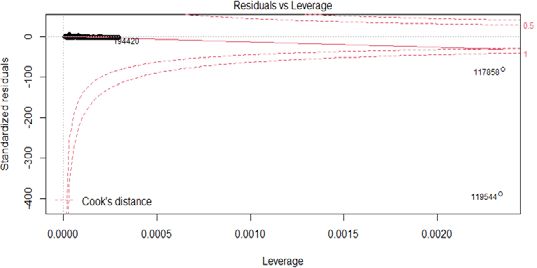
(IJACSA) International Journal of Advanced Computer Science and Applications,
 Vol. 13, No. 1, 2022

 Fig. 4. Linearity.

 Fig. 7. Residuals vs Leverage.

 7) Cook’s distance: This score considers the combined
 values of leverage and residual parameters to determine an
 influential value. Regression analysis results will change with
 the inclusion or exclusion of influential value. An influential
 value has a larger residual. In linear regression analysis all
 outliers (or extreme data points) are not significant. Residuals
 show nearly even spread along the range of predictors. The
 Fig. 5. QQ Plots. red line in the plot is nearly horizontal with similar dense
 distribution of points on either side. We can assume
 3) Homoscedasticity: Fig. 6 shows how residuals are homogeneity of variance.
evenly spread along the range of predictors. The red line in the
plot is nearly horizontal with similar dense distribution of
points on either side. We can assume homogeneity of variance.

 Fig. 6. Homoscedasticity.

 4) Durbin-Watson (DW) test: DW test examines whether Fig. 8. Cooks Distance.
the error terms are autocorrelated. Null hypothesis states that
no autocorrelation exists. The statistical DW test was Cook's distance aids in determining the influential value.
 Here the thumb rule is, observations will have larger influence,
performed and based on the p-value, we conclude that no
 if Cook's distance is more than 4/(n - p - 1) [14]. In the
autocorrelation exists. Statistical DW test yields the test result expression n represents the count of observations and p- the
as ~1.9, which means, no autocorrelation exists. Hence, this number of predictor variables.
assumption is validated.
 5) VIF for multicollinearity: On examining variable In the given data, Cook's distance is too small as depicted
inflation factors for predictor variables, it was found that they in Fig. 8 and does not have significant influence on regression
 analysis. However, outliers, if any, must be detected and
do not exceed 5, hence, no multi-collinearity exists in the data
 suitably handled.
set, which means, and the assumption of no multicollinearity
is validated. C. Multiple Linear Regression Model
 6) Residual v/s Leverage: The most influential 3 values MLR is a statistical approach for predicting the output of a
are shown on the plot in Fig. 7; however, they can be dependent variable by considering multiple independent
exceptions, or, outliers. In this case, data does not present any variables [15]. MLR is capable of building a linear relationship
high influence points. between predictor variables and response values. Data is
 collected from the Intel Research Labs. Initially to eliminate
 noisy values, data pre-processing is done, avoiding reduction in
 prediction accuracy. Now, pre-processed data must be divided

 257 | P a g e
 www.ijacsa.thesai.org

(IJACSA) International Journal of Advanced Computer Science and Applications,
 Vol. 13, No. 1, 2022

into training and test data. The proposed algorithm needs to be Usually squared values of errors are taken before averaging,
trained utilizing training data for establishing relationship with since RMSE gives relatively more weight to larger errors.
several parameters. The final model will predict outcome of Hence, RMSE is most suitable for large number of undesirable
any new given data set containing data for same independent errors. Though RMSE penalizes larger errors, MAE has better
variables. interpretability, hence is considered.
 1) Evaluation parameters: The Model built is evaluated The size of the dataset was decided by extracting random
using various statistical metrics as listed below. samples from the master dataset which keeps the distribution at
 a) R-square: In MLR models r-square is used to a defined significance level. Basically, in order to achieve
 higher statistical significance, a machine learning model must
measure a goodness-of-fit. Purpose of using this statistic is to
 be trained for larger dataset. But to save time sub-samples are
judge how independent variables can mutually explain the
dependent variable variance in percentage. selected maintaining other statistics same. Data distribution is
 Variance explained by full model
 fairly normal.
R − Square = (7)
 Total Variance
 IV. RESULTS
 R-square increases every time a new independent variable All data pre-processing, exploratory analysis, Model build,
is added to the Model. While a higher R-square is desirable, tune and validation were performed using R language. In order
one has to vary about over-inflating the results and overfitting to predict humidity, data pre- processing followed by multiple
the Model. linear regression method was used. Existing data mining
 b) Adjusted R-square: In regression Models, this methods worked on homogeneous data, but the presented
statistic is used for comparing the goodness-of-fit with model is capable of handling heterogeneous data. The model
independent variables. The number of terms in the Model is performance was evaluated by using statistical metrics like R2,
adjusted with adjusted r-square. Importantly this parameter is MAE, RMSE, etc.
mainly used to check an improvement in the Model fit with a 1) Intel dataset: For experimentation, freely available
new term. The adjusted R-squared value will automatically Intel Lab dataset [16] was used. This dataset has nearly 2.3
decrease whenever the new term fails to enhance the model fit million records collected by deploying 54 sensors in the Intel
by an adequate amount. Berkeley Research lab. Sensors used were Mica2Dot, capable
 In our situation, r-square and adjusted-r-square are above- of collecting time-stamped weather information. The values
average values, and acceptable. are recorded by in-network query processing TinyDB system
 c) Mean Absolute Error (MAE): While predicting a set and these are recorded once every 31 seconds with humidity,
of values MAE is used to measure errors average magnitude, temperature, light and voltage as key variables. The dataset
independent of direction. format is given by: date, time, epoch, mote ID, temperature,
 With all equal weighted individual differences, MEA is humidity, light, and voltage. All the sensors are numbered
computed as the test samples average parameter, considering with ids ranging from 1-54. Some sensor’s values are missing
the absolute differences between actual and prediction or approximated. These measured variables are represented as,
observations. temperature in degrees Celsius, humidity ranging from 0-100%
 n and its temperature corrected relative humidity. Light is
 1
MAE = � �yj − y� j � (8) recorded in Lux (1 Lux is equivalent to moonlight, 400 Lux
 n j=1
 corresponds to a bright office, and 100,000 Lux is equivalent
 Where, n – Number of samples, yj -Expected value and y� j - to full sunlight). Voltage is in the range 2-3, measured in volts.
Predicted value. Lithium ion cell batteries were used for providing constant
 d) Root Mean Squared Error (RMSE): RMSE is a voltage to sensors for their lifetime. It is observed that voltage
squared output used for measuring average score of error. variations are highly correlated with temperature.
 It’s the square root of the average of squared differences 2) Model Results and Evaluation Metrics
between prediction and actual observation. a) R-square: 0.692: Higher the R-square value, better it
 is. This statistical value shows variation between the
 n 2 dependent and independent variables. R-square is 0.692,
 1
RMSE = � � �yj − y� j � (9) which is considered a good-fit. Independent variables are able
 n j=1
 to explain a large amount of variance in dependent variable.
 Where, n – Number of samples, yj -Expected value and y� j - p-value : Model is statistically significant.
Predicted value.
 b) Metrics: As observed in Table I, average error is
 MAE and RMSE values lie between 0 and ∞, and are ~11%, hence we say Model is accurate upto 89%. MAE and
independent of the direction of errors. Both the metrics can be RMSE are very small, hence our Model is very good;
used for error prediction, expressing the variables in the predictions generated from this Model will be very accurate.
interest of values units. For efficient modeling lower values are
preferred, since both MAE and RMSE yield negative results. c) Residuals: Table II gives residuals statistics for
 outliers treatment.

 258 | P a g e
 www.ijacsa.thesai.org

(IJACSA) International Journal of Advanced Computer Science and Applications,
 Vol. 13, No. 1, 2022

 TABLE I. STATISTICS OF RESIDUALS Machine Learning techniques are used for weather prediction,
MAE MSE RMSE MAPE
 and MLR algorithm is built using temperature, humidity, light
 and voltage as the key variables. We have evaluated the Model
0.113799 0.03070434 0.17522655 Inf. and model results are documented above. The resultant model
 can predict with high degree of accuracy and can be expanded
 TABLE II. STATISTICS OF RESIDUALS FOR TREATING OUTLIERS for further work. Values of statistical parameters indicate that
 the proposed model is statistically more significant compared
Min 1Q Median 3Q Max
 to other existing techniques.
-0.93682 -0.08049 0.00572 0..08174 0.97949
 REFERENCES
 d) Coefficients: Table III lists the model coefficients for [1] Mohd Fauzi Othmana , Khairunnisa Shazalib, 2012,’ Wireless Sensor
 Network Applications: A Study in Environment Monitoring System’,
variables temperature, voltage, light and their correlations. International Symposium on Robotics and Intelligent Sensors 2012 (IR
 IS 2012) , Procedia Engineering 41 ( 2012 ) 1204 – 1210.
 TABLE III. MODEL COEFFICIENTS
 [2] Munmun B, Tanni D, Sayantanu B (2018), ‘Weather forecast prediction:
 Std. an integrated approach for analyzing and measuring weather data’. Int J
Variables Estimate t Value Pr(>|t|) Computer Appl. https://doi.org/10.5120/ijca2018918265.
 Error
 < 2e-16 [3] Kothapalli S, Totad SG (2017), ’A real-time weather forecasting and
Intercept 0.936820 0.002421 386.889 analysis’. In: IEEE international conference on power, control, signals
 ***
 and instrumentation engineering (ICPCSI-2017), pp 1567–1570.
 < 2e-16
Temperature -0.919190 0.003173 -289.665 [4] Almgren K, Alshahrani S, Lee J (2019),’Weather data analysis using
 ***
 hadoop to mitigate event planning disasters’.
 < 2e-16
Voltage -0.134744 0.003269 -41.224 https://scholarworks.bridgeport.edu/xmlui/handle/123456789/1105
 ***
 Accessed 1 Feb 2019.
 < 2e-16
Light -0.080437 0.007696 -41.224 [5] N. Krishnaveni, A. Padma, 2020, ‘Weather forecast prediction and
 ***
 analysis using sprint algorithm’, © Springer-Verlag GmbH Germany,