A Review of EEG Signal Features and Their Application in Driver Drowsiness Detection Systems - MDPI
←
→
Page content transcription
If your browser does not render page correctly, please read the page content below
sensors
Review
A Review of EEG Signal Features and Their Application in
Driver Drowsiness Detection Systems
Igor Stancin, Mario Cifrek                   and Alan Jovic *

                                            Faculty of Electrical Engineering and Computing, University of Zagreb, Unska 3, 10000 Zagreb, Croatia;
                                            igor.stancin@fer.hr (I.S.); mario.cifrek@fer.hr (M.C.)
                                            * Correspondence: alan.jovic@fer.hr

                                            Abstract: Detecting drowsiness in drivers, especially multi-level drowsiness, is a difficult problem
                                            that is often approached using neurophysiological signals as the basis for building a reliable system.
                                            In this context, electroencephalogram (EEG) signals are the most important source of data to achieve
                                            successful detection. In this paper, we first review EEG signal features used in the literature for a
                                            variety of tasks, then we focus on reviewing the applications of EEG features and deep learning
                                            approaches in driver drowsiness detection, and finally we discuss the open challenges and opportu-
                                            nities in improving driver drowsiness detection based on EEG. We show that the number of studies
                                            on driver drowsiness detection systems has increased in recent years and that future systems need
                                            to consider the wide variety of EEG signal features and deep learning approaches to increase the
                                            accuracy of detection.

                                            Keywords: drowsiness detection; EEG features; feature extraction; machine learning; drowsiness
                                            classification; fatigue detection; deep learning


Citation: Stancin, I.; Cifrek, M.; Jovic,
A. A Review of EEG Signal Features          1. Introduction
and Their Application in Driver                  Many industries (manufacturing, logistics, transport, emergency ambulance, and
Drowsiness Detection Systems.
                                            similar) run their operations 24/7, meaning their workers work in shifts. Working in shifts
Sensors 2021, 21, 3786. https://
                                            causes misalignment with the internal biological circadian rhythm of many individuals,
doi.org/10.3390/s21113786
                                            which can lead to sleeping disorders, drowsiness, fatigue, mood disturbances, and other
                                            long-term health problems [1–4]. Besides misalignment of the internal circadian rhythms
Academic Editor: Giovanni Sparacino
                                            with a work shift, sleep deprivation and prolonged physical or mental activity can also
                                            cause drowsiness [5–7]. Drowsiness increases the risk of accidents at the workplace [8–10],
Received: 29 March 2021
Accepted: 28 May 2021
                                            and it is one of the main risk factors in road and air traffic accidents per reports from
Published: 30 May 2021
                                            NASA [11] and the US National Transportation Safety Board [12].
                                                 Drowsiness is the intermediate state between awareness and sleep [13–15]. Terms like
Publisher’s Note: MDPI stays neutral
                                            tiredness and sleepiness are used as synonyms for drowsiness [16–18]. Some researchers
with regard to jurisdictional claims in
                                            also use fatigue as synonymous with drowsiness [19,20]. Definitions and differences
published maps and institutional affil-     between drowsiness and fatigue are addressed in many research papers [21–23]. The main
iations.                                    difference between the two states is that short rest abates fatigue, while it aggravates
                                            drowsiness [24]. However, although the definitions are different, drowsiness and fatigue
                                            show similar behavior in terms of features measured from electroencephalogram (EEG)
                                            signal [25–28]. Because of this fact, in this review paper, we consider all the research
Copyright: © 2021 by the authors.
                                            papers whose topic was drowsiness, sleepiness, or fatigue, and we make no distinction
Licensee MDPI, Basel, Switzerland.
                                            among them.
This article is an open access article
                                                 The maximum number of hours that professional drivers are allowed to drive in a
distributed under the terms and             day is limited, yet drowsiness is still a major problem in traffic. A system for drowsiness
conditions of the Creative Commons          detection with early warnings could address this problem. The most commonly used meth-
Attribution (CC BY) license (https://       ods for drowsiness detection are self-assessment of drowsiness, driving events measures,
creativecommons.org/licenses/by/            eye-tracking measures, and EEG measures. Among these methods, drowsiness detection
4.0/).                                      systems based on the EEG signal show the most promising results [18,29].

Sensors 2021, 21, 3786. https://doi.org/10.3390/s21113786                                                      https://www.mdpi.com/journal/sensors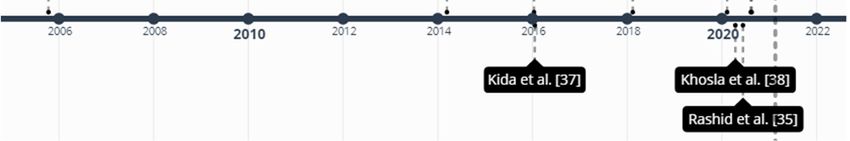
Sensors 2021, 21, 3786                                                                                            2 of 29

                              Brain neural network is a nonlinear dissipative system, i.e., it is a non-stationary
                         system with a nonlinear relationship between causes and effects [30]. One way to ana-
                         lyze brain neural network is through feature extraction from the EEG signal. The most
                         used techniques for feature extraction are linear, such as Fast Fourier Transform (FFT).
                         Although it is a linear method, FFT also assumes that the amplitudes of all frequency
                         components are constant over time, which is not the case with brain oscillations, since
                         they are non-stationary. Because of the complexity of brain dynamics, there is a need
                         for feature extraction methods that can properly take into account the nonlinearity and
                         non-stationarity of brain dynamics. With an increase of computational power in recent
                         years, many researchers work on improving the feature extraction methods, and there is a
                         growing number of various features extracted from the EEG signal.
                              This paper aims to review the features extracted from the EEG signal and the appli-
                         cations of these features to the problem of driver drowsiness detection. We review the
                         features since the large number of features described in the literature makes it difficult to
                         understand their interrelationships, and also makes it difficult to choose the right ones
                         for the given problem. To our knowledge, there is no similar review work that covers all
                         the features discussed in this review. After the EEG features review, we continue with the
                         review of driver drowsiness detection systems based on EEG. The main goal is to gain
                         insight into the most commonly used EEG features and recent deep learning approaches for
                         drowsiness detection, which would allow us to identify possibilities for further improve-
                         ments of drowsiness detection systems. Finally, the main contributions of our work are
                         the following: (1) Comprehensive review, systematization, and a brief introduction of the
                         existing features of the EEG signal, (2) comprehensive review of the drowsiness detection
                         systems based on the EEG signal, (3) comprehensive review of the existing similar reviews,
                         and (4) discussion of various potential ways to improve the state of the art of drowsiness
                         detection systems.
                              The paper is organized as follows: In Section 2, we present the overview of the existing
                         review papers that are close to the topic of this paper, Section 3 provides the overview of the
                         different features extracted from the EEG signal, Section 4 reviews the papers dealing with
                         driver drowsiness detection systems, Section 5 provides a discussion about the features
                         and drowsiness detection systems, and Section 6 brings the future directions of research
                         and concludes the paper.
                              The search for the relevant papers included in our paper was done in the Web of
                         Science Core Collection database. The search queries used were: (1) In Section 2.1—
                         “{review, overview} {time, frequency, spectral, nonlinear, fractal, entropy, spatial, temporal,
                         network, complex network} EEG features“, (2) in Section 2.2—“{review, overview} driver
                         {drowsiness, sleepiness, fatigue} {detection, classification}”, (3) in Section 3—“ EEG feature”, (4) in Section 4—“EEG driver {‘’, deep learning, neural network}
                         {drowsiness, sleepiness, fatigue} {detection, classification}”. Beyond the mentioned queries,
                         when appropriate, we also reviewed the papers cited in the results obtained through the
                         query. Additional constraints for papers in Section 4 were: (1) They had to be published in
                         a scientific journal, (2) they had to be published in 2010 or later, 2) at least three citations
                         per year since the paper was published, (3) papers from 2020 or 2021 were also considered
                         with less than three citations per year, but published in Q1 journals, and (4) the number of
                         participants in the study experiment had to be greater than 10. The goal of these constraints
                         was to ensure that only high quality and relevant papers were included in our study.

                         2. Related Work
                         2.1. Reviews of the EEG Signal Features
                              Stam [30] in his seminal review paper about the nonlinear dynamical analysis of the
                         EEG and magnetoencephalogram (MEG) signals included more than 20 nonlinear and
                         spatiotemporal features (e.g., correlation dimension, Lyapunov exponent, phase synchro-
                         nization). The theoretical background of these features and dynamical systems were also
                         covered. The paper gave an overview of the other research works that include explanations
Sensors 2021, 21, 3786 3 of 29
of the features from the fields of normal resting-state EEG, sleep, epilepsy, psychiatric
diseases, normal cognition, distributed cognition, and dementia. The main drawback of the
paper nowadays is that it is somewhat dated (from 2005) because additional approaches
have been introduced in the meantime. Ma et al. [31] reviewed the most-used fractal-based
features and entropies for the EEG signal analysis, and focused on the application of these
features to sleep analysis. The authors concluded that using fractal or entropy methods may
facilitate automatic sleep classification. Keshmiri [32], in a recent paper, provided a review
on the usage of entropy in the fields of altered state of consciousness and brain aging. The
author’s work is mostly domain-specific, as it emphasizes incremental findings in each area
of research rather than the specific types of entropies that were utilized in the reviewed
research papers. Sun et al. [33] reviewed the complexity features in mild cognitive impair-
ment and Alzheimer’s disease. They described the usage of five time-domain entropies,
three frequency-domain entropies, and four chaos theory-based complexity measures.
Motamedi-Fakhr et al. [34], in their review paper, provided an overview of more
than 15 most-used features and methods (e.g., Hjorth parameters, coherence analysis,
short-time Fourier transform, wavelet transform) for human sleep analysis. The features
were classified into temporal, spectral, time-frequency, and nonlinear features. Besides
these features, they also reviewed the research papers about sleep stages classification.
Rashid et al. [35] reviewed the current status, challenges, and possible solutions for EEG-
based brain-computer interface. Within their work, they also briefly discussed the most
used features for brain–computer interfaces classified into time domain, frequency domain,
time-frequency domain, and spatial domain.
Bastos and Schoffelen [36] provided a tutorial review of methods for functional con-
nectivity analysis. The authors aimed to provide an intuitive explanation of how functional
connectivity measures work and highlighted five interpretational caveats: The common
reference problem, the signal-to-noise ratio, the volume conduction problem, the common
input problem, and the sample size problem. Kida et al. [37], in their recent review paper,
provided the definition, computation, short history, and pros and cons of the connec-
tivity and complex network analysis applied to EEG/MEG signals. The authors briefly
described the recent developments in the source reconstruction algorithms essential for the
source-space connectivity and network analysis.
Khosla et al. [38], in their review, covered the applications of the EEG signals based on
computer-aided technologies, ranging from the diagnosis of various neurological disorders
such as epilepsy, major depressive disorder, alcohol use disorder, and dementia to the
monitoring of other applications such as motor imagery, identity authentication, emotion
recognition, sleep stage classification, eye state detection, and drowsiness monitoring. By
reviewing these EEG signal-based applications, the authors listed features observed in
these papers (without explanations), publicly available databases, preprocessing methods,
feature selection methods, and used classification models. For the application of drowsi-
ness monitoring, the authors reviewed only three papers, while other applications were
better covered.
Ismail and Karwowski [39] overview paper dealt with a graph theory-based modeling
of functional brain connectivity based on the EEG signal in the context of neuroergonomics.
The authors concluded that the graph theory measures have attracted increasing attention
in recent years, with the highest frequency of publications in 2018. They reviewed 20 graph
theory-based measures and stated that the clustering coefficient and characteristic path
length were mostly used in this domain.
Figure 1 shows the reviews presented in this section in chronological order of publication.attention in recent years, with the highest frequency of publications in 2018. They re‐
viewed 20 graph theory‐based measures and stated that the clustering coefficient and
Sensors 2021, 21, 3786 characteristic path length were mostly used in this domain. 4 of 29
Figure 1 shows the reviews presented in this section in chronological order of publi‐
cation.
Figure 1.
Figure 1. Chronologically
Chronologically ordered
ordered reviews
reviews of
of the
the EEG
EEG signal
signal features.
features.
2.2. Reviews
2.2. Reviews of of the
the Driver Drowsiness Detection
Driver Drowsiness Detection
Lal and
Lal and Craig
Craig[18],[18],inintheir
theirreview
reviewofof driver
driver drowsiness
drowsiness systems,
systems, discussed
discussed the the con‐
concept
cept
of of fatigue
fatigue and summarized
and summarized the psychophysiological
the psychophysiological representation
representation of driver
of driver fatigue.
fatigue. They
concluded that most studies had found a correlation of theta and delta activity withwith
They concluded that most studies had found a correlation of theta and delta activity the
the transition
transition to fatigue.
to fatigue.
Lenne and
Lenne and Jacobs
Jacobs[40],
[40],inintheir
theirreview
review paper,
paper, assessed
assessed thethe recent
recentdevelopments
developments in thein
detection and prediction of drowsiness‐related driving
the detection and prediction of drowsiness-related driving events. The driving eventsevents. The driving events ob‐
served were
observed were thethe number
numberofofline linecrossings,
crossings,the thestandard
standarddeviation
deviation of of lateral position, the
lateral position, the
variability of
variability of lateral
lateral position,
position, steering
steering wheel
wheel variability,
variability, speed
speed adjustments,
adjustments, and and similar
similar
events. The
events. The authors concluded that
authors concluded that these
these driving
driving performance
performance measuresmeasures correlate
correlate with
with
drowsiness in the experimental settings, although they stipulated
drowsiness in the experimental settings, although they stipulated that the new findings that the new findings
from on-road
on‐roadstudies
studiesshow showa adifferent
different impact
impact on on performance
performance measures.
measures. Doudou
Doudou et al.et[41]
al.
[41] reviewed
reviewed the vehicle‐based,
the vehicle-based, video‐based,
video-based, and and physiological
physiological signals‐based
signals-based techniques
techniques for
for drowsiness
drowsiness detection.
detection. They Theyalsoalso reviewed
reviewed the the available
available commercial
commercial market
market solutions
solutions for
for drowsiness
drowsiness detection.
detection. When When it comes
it comes to theto EEG
the EEGsignal signal drowsiness
drowsiness detection,
detection, the au‐
the authors
thors included
included six paperssix papers that consider
that consider frequency‐domain
frequency-domain features features
in thisin this field.
field.
Sahayadhas et al. [42] reviewed reviewed vehicle-based
vehicle‐based measures, behavior-basedbehavior‐based measures,
and physiological measures for for driver drowsiness
drowsiness detection.
detection. The section on physiological
physiological
measures included
included 12 12papers
paperswith withonlyonlyfrequency‐domain
frequency-domain features.
features. Sikander
SikanderandandAnwarAn-
war [43] reviewed
[43] reviewed drowsiness
drowsiness detection
detection methodsmethods and categorized
and categorized themthem into groups—sub‐
into five five groups—
subjective reporting,
jective reporting, driverdriver biological
biological features,
features, driverdriver physical
physical features,
features, vehicular
vehicular fea-
features
tures
whilewhile
driving,driving, and hybrid
and hybrid features.features.
WhenWhen it comesit comes to drowsiness
to drowsiness detection
detection usingusing
EEG
EEG
signals,signals, the authors
the authors focused
focused moremore on explaining
on explaining frequency-domain
frequency‐domain features
features used usedfor
for drowsiness detection rather than presenting research that
drowsiness detection rather than presenting research that had already been done in this had already been done in
this
field.field.
Chowdhury et al. [44] reviewed reviewed different
different physiological
physiological sensors sensors applied
applied to to driver
driver
drowsiness
drowsiness detection.
detection.Observed
Observed physiological
physiological methods
methods for measuring
for measuring drowsiness included
drowsiness in‐
electrocardiogram (ECG), respiratory belt, EEG, electrooculogram
cluded electrocardiogram (ECG), respiratory belt, EEG, electrooculogram (EOG), electro‐ (EOG), electromyogram
(EMG),
myogram galvanic
(EMG),skin response
galvanic skin(GSR),
responseskin(GSR),
temperature, and hybridand
skin temperature, techniques. Related to
hybrid techniques.
EEG methods, the authors included papers based on
Related to EEG methods, the authors included papers based on the spectral power the spectral power features, event-
fea‐
related potentials, and entropies. The authors also discussed
tures, event‐related potentials, and entropies. The authors also discussed different mate‐ different materials used for
dry
rialselectrodes
used for dry andelectrodes
the problem andofthe measurement
problem of intrusiveness
measurementfor the drivers.for the driv‐
intrusiveness
ers. Balandong et al. [45] split driver drowsiness detection systems into six categories based
on the used technique—(1) subjective measures, (2) vehicle-based measures, (3) driver’s
behavior-based system, (4) mathematical models of sleep–wake dynamics, (5) human
physiological signal-based systems, and (6) hybrid systems. The authors emphasized
human physiological signal-based systems, but only the systems that rely on a limited
number of EEG electrodes, as these kinds of systems are more practical for real-world
applications. The authors concluded that the best results were obtained when the problemBalandong et al. [45] split driver drowsiness detection systems into six categories
based on the used technique—(1) subjective measures, (2) vehicle‐based measures, (3)
driver’s behavior‐based system, (4) mathematical models of sleep–wake dynamics, (5) hu‐
man physiological signal‐based systems, and (6) hybrid systems. The authors emphasized
Sensors 2021, 21, 3786
human physiological signal‐based systems, but only the systems that rely on a limited 5 of 29
number of EEG electrodes, as these kinds of systems are more practical for real‐world
applications. The authors concluded that the best results were obtained when the problem
was observed as a binary classification problem and that the fusion of the EEG features
was observed
with as a binarysignals
other physiological classification problem
should lead and thataccuracy.
to improved the fusion of the EEG features
withOther
other review
physiological
paperssignals should
of driver lead tosystems
drowsiness improved areaccuracy.
specialized for a certain aspect
Other review papers of driver drowsiness systems
of the field, e.g., Hu and Lodewijsk [46] focused on differentiatingare specialized for a certain
the detection aspect
of passive
of the field, e.g., Hu and Lodewijsk [46] focused on differentiating the detection
fatigue, active fatigue, and sleepiness based on physiological signals, subjective assess‐ of passive
fatigue,
ment, active fatigue,
driving behavior,and sleepiness
and based onSoares
ocular metrics, physiological signals,
et al. [47] subjective
studied assessment,
simulator experi‐
driving
ments forbehavior,
drowsiness anddetection,
ocular metrics, Soares
Bier et al. et al.
[48] put [47]on
focus studied simulator experiments
the monotony‐related fatigue,
for drowsiness
and Philips et al.detection, Bier et
[49] studied al. [48] putactions
operational focus on theoptimal
(e.g., monotony-related fatigue,
staff, optimal and
schedule
Philips et al. [49] studied operational actions
design) that reduce risk of drowsiness occurrence. (e.g., optimal staff, optimal schedule design)
that Figure
reduce 2risk of drowsiness
shows the reviews occurrence.
presented in this section in chronological order of publi‐
Figure
cation. 2 shows the reviews presented in this section in chronological order of publication.
Figure
Figure 2.
2. Chronologically
Chronologically ordered
ordered reviews
reviews of
of driver
driver drowsiness
drowsiness detection
detection methods.
methods.
3.
3. EEG
EEG Features
Features
The
The purpose
purpose of of this
this section
section isis to
to introduce
introduce features
features that
that researchers
researchers extract
extract from
from thethe
EEG signal. We will not go into the details of the computation
EEG signal. We will not go into the details of the computation for each feature. for each feature. For For
the
readers whowho
the readers are interested in theindetailed
are interested computation
the detailed for each
computation for feature, we suggest
each feature, read‐
we suggest
ing the cited papers. Instead, the main idea is to present, with a brief explanation,
reading the cited papers. Instead, the main idea is to present, with a brief explanation, as as many
features as possible,
many features whichwhich
as possible, will later
will allow us to us
later allow identify opportunities
to identify opportunities for further im‐
for further
provements
improvements in the area of driver drowsiness detection. Tables 1 and 2 show the list of all
in the area of driver drowsiness detection. Tables 1 and 2 show the list of all
the
the features
features introduced
introduced in in the
the following
following subsections.
subsections. In In the
the rest
rest ofof this
this Section,
Section, wewe will
will use
use
bold
bold letters for the
letters for thefirst
firstoccurrence
occurrenceofofa particular
a particular feature
feature name
name andand italic
italic letters
letters for first
for the the
first occurrence
occurrence of a particular
of a particular feature
feature transformation
transformation or extraction
or extraction methodmethod
name. name.
3.1. Time, Frequency and Time-Frequency Domain Features
3.1.1. Time-Domain Features
The simplest features of the EEG signal are statistical features, like mean, median,
variance, standard deviation, skewness, kurtosis, and similar [50]. Zero-crossing rate
(ZCR) [51] is not a statistical feature, yet it is also a simple feature. It is the number of times
that the signal crosses the x-axis. The period-amplitude analysis is based on the analysis of the
half-waves, i.e., signals between two zero-crossings. With the period amplitude analysis,
one can extract the number of waves, wave duration, peak amplitude, and instantaneous
frequency (IF) (based only on the single observed half-wave) [52].
Hjorth parameters are features that are based on the variance of the derivatives of the
EEG signal. Mobility, activity, and complexity [53] are the first three derivatives of the
signal and the most-used Hjorth parameters. Mean absolute value of mobility, activity, and
complexity can also be used as a features [54]. K-complex [55] is a characteristic waveform
of the EEG signal that occurs in stage two of the non-rapid eye movement sleep phase.
Energy (E) of the signal is the sum of the squares of amplitude.Sensors 2021, 21, 3786 6 of 29
3.1.2. Frequency-Domain Features
The power spectral density (PSD) of the signal, which is the base for calculation
of the frequency domain features, can be calculated with several parametric and non-
parametric methods. Non-parametric methods are used more often and include methods
like Fourier transform (usually calculated with Fast Fourier transform algorithm, FFT [56]),
Welch’s method [57], or Thompson multitaper method [58]. Examples of parametric methods
for the PSD estimation are the autoregressive (AR) models [59], multivariate autoregressive
models [60], or the autoregressive-moving average (ARMA) models [61]. The non-parametric
models have a more widespread usage, because there is no need for selecting parameters
such as the model’s order, which is the case for autoregressive models.
Statistical features like mean, median, variance, standard deviation, skewness, kur-
tosis, and similar are also used in the frequency domain. Relative powers of the certain
frequency bands are the most used frequency-domain features in all fields of analysis of
the EEG signals. The most commonly used frequency bands are delta (δ, 0.5–4 Hz), theta
(θ, 4–8 Hz), alpha (α, 8–12 Hz), beta (β, 12–30 Hz), and gamma (γ, >30 Hz), band. There
is also the sigma band (σ, 12–14 Hz) that is sometimes called sleep spindles [62]. Several
ratios between frequency bands are widely used as features in the EEG signal analysis, i.e.,
θ/α [63], β/α [63], (θ + α)/β [64], θ/β [64], (θ + α)/(α + β) [64], γ/δ [65] and (γ + β)/(δ +
α) [65].
Table 1. The list of time-domain, frequency domain and nonlinear features reviewed in this work.
Group Feature Name Abbr. Group Feature Name Abbr.
Mean θ/β
Frequency-domain
Median (θ + α)/(α + β)
Variance γ/δ
Standard deviation (γ + β)/(δ + α)
Skewness Reflection coefficients
Kurtosis Partial correlation coefficient
Time-domain
Zero-crossing rate ZCR Wavelet coefficients
Number of waves Phase coupling
Wave duration Hurst exponent H
Peak amplitude Renyi scaling exponent
Instantaneous frequency IF Renyi gener. dim. multifractals
Hjorth parameters Capacity dimension D0 D0
Mobility Information dimension D1 D1
Activity Correlation dimension D2 D2
Complexity Katz fractal dimension KFD
K-complex Petrosian fractal dimension PFD
Energy E Higuchi fractal dimension HFD
Mean Fractal spectrum
Nonlinear
Median Lyapunov exponents LE
Variance Lempel-Ziv complexity LZC
Standard deviation Central tendency measure CTM
Frequency-domain
Skewness Auto-mutual information AMI
Kurtosis Temporal irreversibility
Delta δ Recurrence rate RR
Theta θ Determinism Det
Alpha α Laminarity Lam
Beta β Average diagonal line length L
Gamma γ Maximum length of diagonal Lmax
Sigma σ Max. length of vertical lines Vmax
θ/α Trapping time TT
β/α Divergence Div
(θ + α)/β Entropy of recurrence plot ENTRSensors 2021, 21, 3786 7 of 29
Table 2. The list of entropies, undirected and directed spatiotemporal (spt.), and complex network features reviewed in
this work.
Group Feature Name Abbr. Group Feature Name Abbr.
Shannon entropy Imaginary component of Coh
Renyi’s entropy Phase-lag index PLI
Tsallis entropy Weighted phase lag index wPLI
Undirected spt.
Kraskov entropy KE Debiased weighted PLI dwPLI
Spectral entropy SEN Pairwise phase consistency PPC
Quadratic Renyi’s SEN QRSEN Generalized synchronization
Response entropy RE Synchronization likelihood SL
State entropy SE Mutual information MI
Wavelet entropy WE Mutual information in freq. MIF
Tsallis wavelet entropy TWE Cross-RQA
Rényi’s wavelet entropy RWE Correlation length ξKLD
Directed spt.
Hilbert-Huang SEN HHSE Granger causality
Log energy entropy LogEn Spectral Granger causality
Multiresolution entropy Phase slope index PSI
Entropies
Kolmogorov’s entropy Number of vertices
Nonlinear forecasting entropy Number of edges
Maximum-likelihood entropy Degree D
Coarse-grained entropy Mean degree
Correntropy CoE Degree distribution
Approximate entropy ApEn Degree correlation r
Sample entropy SampEn Kappa k
Quadratic sample entropy QSE Clustering coefficiet
Multiscale entropy MSE Transitivity
Modified multiscale entropy MMSE Motif
Complex networks
Composite multiscale entropy CMSE Characteristic path length
Permutation entropy PE Small worldness
Renyi’s permutation entropy RPE Assortativity
Permutation Rényi entropy PEr Efficiency
Multivariate PE MvPE Local efficiency
Tsallis permutation entropy TPE Global efficiency
Dispersion entropy DisE Modularity
Amplitude-aware PE AAPE Centrality degree
Bubble entropy BE Closesness centrality
Differential entropy DifE Eigenvalue centrality
Fuzzy entropy FuzzyEn Betweenness centrality
Transfer entropy TrEn Diameter d
Undirected spt.
Coherence Eccentricity Ecc
Partial coherence Hubs
Phase coherence Rich club
Phase-locking value PLV Leaf fraction
Coherency Coh Hierarchy Th
The frequency domain of the signal can also be obtained using wavelet decomposi-
tion [66,67] and matching pursuit decomposition [68,69] methods. Unlike Fourier transform,
which decomposes a signal into sinusoids, wavelet decomposition uses an underlying
mother wavelet function for decomposition, and matching pursuit decomposition uses the
dictionaries of signals to find the best fit for the signal.
From autoregressive models, one can extract features such as reflection coefficients
or partial correlation coefficients. Wavelet coefficients obtained after applying wavelet
decomposition can also be used as features. PSD is usually used to obtain the second-order
statistics of the EEG signal. However, one can also consider the higher-order spectrum. ForSensors 2021, 21, 3786 8 of 29
example, phase coupling [70] of different frequency components can be obtained with the
higher-order spectral analysis.
3.1.3. Time-Frequency Features
The analysis of the EEG signal in the domains of time and frequency simultaneously is
a powerful tool, since the EEG signal is a non-stationary signal [71,72]. The most important
component of time-frequency domain analysis is the possibility to observe changes in the
frequency over time. Short-time Fourier transform (STFT) is the simplest function that
uses uniform separation of the observed signal and calculates its frequency components.
A spectrogram [71] can be obtained with the application of STFT. Wavelet transform [73]
is the usual alternative method to spectrogram that also provides coefficients as features
from the time-frequency domain. The main advantage of wavelet transform compared to
spectrogram is a variable window size, dependent on spectrum frequencies.
3.2. Nonlinear Features
Brain dynamics constitute a complex system. A system is complex when it is con-
structed from many nonlinear subsystems that cannot be separated into smaller subsystems
without changing their dynamical properties. Fractal systems are often used for describing
the brain dynamics measured with the EEG signal. To explain fractal systems, first, we
need to introduce the scaling law. The scaling law is describing (asymptomatically) a
self-similar function F as a function of the scale parameter s, i.e., F (s) ∼ sα . When applied
to a self-affine signal, each axis should be scaled by a different power factor to obtain
statistically equivalent changes in both directions. If s is used in the x-axis direction, then
s0 = s H should be used in the y-axis direction. The power factor H is called the Hurst
exponent [74,75]. The Hurst exponent is a measure of long-term memory of the signal and
is related to the fractal dimension with the equation D0 = 2 − H for self-similar time-series,
where fractal dimension D0 is defined in the next paragraph. Time-series q is monofractal if
it is linearly interdependent with its Renyi scaling exponent τ (q), otherwise, it is multifrac-
tal. The Renyi generalized dimension of multifractals is defined as D (q) = τ (q)/(q − 1).
For more detailed explanations about fractality and multifractality of the time-series, we
refer the reader to [76–78].
In EEG signal analysis, all fractal dimensions are estimated based on the underlying
attractor (a geometric structure towards which stationary dissipative system gravitates in
its state space) of the signal [79]. In a strict mathematical sense, most time-series have the
one-dimensional support fractal dimension D0 (or capacity dimension or Hausdorff di-
mension) if there are no missing values. Regardless of the value of the D0, the information
dimension D1 and correlation dimension D2 [79–81] can be calculated. The correlational
dimension D2 can be calculated with both monofractal and multifractal approaches. The
Katz fractal dimension (KFD) [82], the Petrosian fractal dimension (PFD) [83], and the
Higuchi fractal dimension (HFD) [84] are different approaches to the estimation of the
fractal dimension. With multifractal time-series analysis, a fractal spectrum consisting of
multiple fractal dimensions can be obtained [85,86].
Methods for fractal time-series analysis can be classified [76] into stationary analysis
methods (such as Fluctuation Analysis [87], Hurst’s Rescaled-Range Analysis [74], and similar),
non-stationary analysis (such as Detrended Fluctuation Analysis [88], Centered Moving Average
Analysis [89], Triangle Total Areas [90], and similar), and multifractal analysis (such as
Wavelet Transform Modulus Maxima [91], Multifractal Detrended Fluctuation Analysis [92], and
similar). Each of these methods provides its own estimation of fractal dimension or scaling
exponent features.
Lyapunov exponents (LE) [93] are measures of the attractor’s complexity. If a system
has at least one positive Lyapunov exponent, then the system can be characterized as a
chaotic dynamical system. A positive Lyapunov exponent points to exponential divergence
of the two nearby trajectories in the attractor over time [94]. Lempel-Ziv complexity
(LZC) [95] is a measure of complexity that binarizes time-series and then searches for theSensors 2021, 21, 3786 9 of 29
occurrence of consecutive binary characters or “words” and counts the number of times
a new “word” is encountered. The Central tendency measure (CTM) [96] is a measure
of the variability of the observed time-series and represents the percentage of points on
the scatter plot that fall into a given radius. Auto-mutual information (AMI) [97] is a
mutual information measure applied to time-delayed versions of the same EEG time-series.
Temporal irreversibility [98] of a time-series implies the influence of nonlinear dynamics,
non-Gaussian noise, or both. It is a statistical property that differs based on the direction
in which time proceeds, e.g., any sequence of measurements has a different probability of
occurrence than its time reverse.
A recurrence plot [99] is a graphical method for the detection of reoccurring patterns
in the time-series. Recurrence quantification analysis (RQA) [100] is a group of algorithms
for the automatic quantification of recurrence plots. RQA is a noise resistant method,
meaning it gives good results even when the signal-to-noise ratio of considered signals
is unfavorable [101]. The recurrence rate (RR) is the probability that a specific state of a
time-series will reoccur. Determinism (Det) is the percentage of points that form diagonal
lines on the recurrence plot and laminarity (Lam) is the percentage of points forming
vertical lines in the recurrence plot. The average diagonal line length (L), maximum
length of diagonal (Lmax), and maximum length of vertical lines (Vmax) are also used
as RQA-based features. Trapping time (TT) is the average vertical line length and it relates
to the predictability of the time-series. Divergence (Div) is the reciprocal value of the
maximal diagonal line length and it can have a trend similar to the positive Lyapunov expo-
nents. Entropy of the recurrence plot (ENTR) reflects the complexity of the deterministic
structure of the system.
3.3. Entropies
Entropy was first introduced to the field of information theory by Shannon in
1948 [102,103]. Shannon’s information entropy is calculated based on the expression
− ∑ p j log p j , where pj is the probability distribution of the observed data. It is used
j
to measure uncertainty or randomness in the observed time-series. There are many
derived variations of information entropy used in EEG analysis. The entropies may be
considered as nonlinear features, but we describe them in a separate subsection due to
their specific calculation.
Rényi’s entropy [104] is defined with the expression − 1−α α ∑ log pαk , where α > 0
and α 6= 1. It is a generalization of Shannon’s entropy in the case of a limited value
of α → 1 . Quadratic Rényi’s entropy (or just Rényi’s entropy) is the case where α = 2.
Tsallis entropy (q-entropy) [105] is a generalization of the Boltzman–Gibbs
entropy from
k q
statistical thermodynamics and is defined with the expression q −1 1 − ∑ pi , where k is a
i
positive constant and q is the non-extensity parameter. For q > 1, the entropy has a more
significant reaction to the events that occur often, whereas for 0 < q < 1, the entropy has a
more significant reaction to rare events.
The three aforementioned entropies can be calculated from the raw EEG signal. Be-
sides that, they are a base for calculating several other entropies in the field of EEG
analysis. Kraskov entropy (KE) [50] is an unbiased estimator of Shannon’s entropy for a
d-dimensional random sample. Spectral entropy (SEN) [106] is calculated with the expres-
sion for Shannon’s entropy based on the normalized PSD of the EEG signal. Quadratic
Renyi’s spectral entropy (QRSEN) [107] is calculated with the usage of Renyi’s entropy
expression, and the difference compared to the spectral entropy is that it gives the higher
weights to the lower frequencies. Commercial M-Entropy Module [108] uses two different
components of spectral entropy—response entropy (RE) and state entropy (SE). State
entropy includes the spectrum between 0.8 and 32 Hz, while response entropy includes the
spectrum between 0.8 and 47 Hz.
Wavelet entropy (WE) [109,110] is somewhat similar to spectral entropy. The differ-
ence is that it is calculated based on the coefficients of the wavelet decomposition of theSensors 2021, 21, 3786 10 of 29
given time-series. There are two generalizations of wavelet entropy—Tsallis wavelet en-
tropy (TWE) and Rényi’s wavelet entropy (RWE) [111]. Hilbert–Huang spectral entropy
(HHSE) [112] applies Shannon’s entropy to the Hilbert–Huang spectrum, which is obtained
by the Hilbert–Huang transform [111,113]. Log energy entropy (LogEn) [114] is similar to
the wavelet entropy, but only uses summation of logarithms of the probabilities. Multires-
olution entropy [115] uses the combination of windowing and wavelet transform for the
detection of changes in parameters that define the observed process (i.e., the parameters of
brain dynamics).
Kolmogorov’s entropy [116] is an embedding entropy and is defined as the sum of
positive Lyapunov exponents. It represents the rate of information loss and a degree
of predictability (regularity) of the attractor. Accurate computation of Kolmogorov’s
entropy is computationally expensive, so several entropies are used for the estimation of
Kolmogorov’s entropy based on the less computationally expensive methods. Nonlinear
forecasting entropy [117] is the estimation of Kolmogorov’s entropy for time-series with
too few points. It is based on the forecasting of the time-series data, i.e., on the correlation
coefficient of the forecasted points with actually observed points. The estimation method is
independent of the forecasting method used. Maximum-likelihood entropy [118] is also
the estimation of Kolmogorov entropy. It is derived with the application of maximum-
likelihood to the correlation integral, which is treated as a probability distribution. Coarse-
grained entropy [119] is an estimation of the attractor’ entropy for cases where standardly
used dimensions, Lyapunov exponents, and Kolmogorov’s entropy are not suitable due to
the high dimensionality of the observed process. Correntropy (CoE) [120] is an estimation
of nonlinear autocorrelation.
Approximate entropy (ApEn) [121] is derived from Kolmogorov’s entropy and its
use in the analysis of the EEG signal (and other physiological signals) is widespread.
It addresses the irregularity of a time-series. Predictable time-series, i.e., time-series
with many repetitive patterns will have a small value of approximate entropy. Sample
entropy (SampEn) [122] was introduced as an improvement to approximate entropy. It
reduces the error of the approximate entropy by eliminating its two disadvantages—(1)
self-matches and (2) dependence on the time-series length. Sample entropy is also an
approximation of signal complexity. Quadratic sample entropy (QSE) [123] is SampEn
insensitive to the data radius parameter r. It allows r to vary as needed to achieve
confident estimates of the conditional probability. Multiscale entropy (MSE) [124] is
a generalization of an entropy measure (such as sample entropy) to different time
scales. Modified multiscale entropy (MMSE) [125] uses the same procedure as MSE,
but replaces coarse-graining with a moving average procedure. Composite multiscale
entropy (CMSE) [126] is a modification of the MSE that tackles the problem of increased
variance and error estimation for short time-series.
Permutation entropy (PE) [127] estimates signal variability based on the repetition of
the ordinal patterns. The algorithm requires parameter m (permutation order) to obtain
ordinal patterns and their probabilities of occurrence. These probabilities are then applied
in Shannon’s entropy expression. Moreover, Renyi’s permutation entropy (RPE) [128],
permutation Rényi entropy (PEr) [129], multivariate permutation entropy (MvPE) [130],
and Tsallis permutation entropy (TPE) [111] can be calculated for the ordinal patterns.
Dispersion entropy (DisE) [131] is a modification of permutation entropy that tackles
the problem of amplitude information loss (since permutation entropy only considers
the order of the amplitude values but not the values themselves). Amplitude-aware
permutation entropy (AAPE) [132] is based on the similar idea of using the value of the
signal with the permutation entropy. Bubble entropy (BE) [133] is similar to permutation
entropy with the main difference in the method used for ranking vectors in the embedding
space. Namely, permutation entropy uses repetition of the ordinal patterns and bubble
entropy uses the number of steps needed to sort a vector with the bubble sort algorithm.
Differential entropy (DifE) [134] calculation is based on Shannon’s entropy expression and
the estimation of the underlying probability density function of time-series. Fuzzy entropySensors 2021, 21, 3786 11 of 29
(FuzzyEn) [135] is based on the concept of fuzzy sets, first introduced by Zadeh [136].
It is similar to sample entropy, but instead of using the Heaviside function for distance
calculation, it uses a fuzzy membership function. Transfer entropy (TrEn) [137] uses
concepts similar to mutual information (see Section 3.4) with the ability to quantify the
exchange of information between two systems. It is an asymmetric measure for information
transfer from process X to process Y, which measures the effect of the past values of
processes X and Y on the present value of process Y.
3.4. Spatiotemporal Features
Features that were introduced above are all calculated based on a single EEG chan-
nel. Since EEG recording devices can have hundreds of channels nowadays, features
that describe the relationship between different channels bring further insight into the
understanding of brain functions. This is the main idea behind the usage of the spatiotem-
poral features—to describe the relationship between different brain regions for particular
states or events. Spatiotemporal features can be divided into two groups—directed and
non-directed. The non-directed ones relate to the synchronization of two or more channels
without any knowledge of the direction, while the directed ones include the causation
between them, i.e., they measure functional connectivity.
3.4.1. Non-Directed Spatiotemporal Features
Coherence [138] is a cross-correlation equivalent in the frequency-domain, i.e., the
cross-correlation of the PSD from two different channels. It reflects the synchronization
of the changes of frequency components between the observed channels. Partial coher-
ence [139] is an adjusted coherence with removed common signal’s linear effect based
on the third channel, which is not physically close to the two observed channels. Phase
coherence [140] is the coherence of the phases of the signals. It was introduced to overcome
the problem of detection of nonlinear dependencies between the two channels.
The phase-locking value (PLV) [141] represents the measure of the transient phase
locking that is completely independent of the signal’s amplitude, which is not the case for
the coherence measure. Coherency [142] is calculated similar to coherence, but without
applying the magnitude operator to the cross-spectral density of two channels. The
obtained complex-valued quantity is called coherency. The imaginary component of
coherency (iCoh) [143] reflects the nonlinear interaction between the two underlying time-
series. Phase-lag index (PLI) [144] is a measure of the asymmetry of the distribution of
phase differences between two signals. It brings improvement compared to the imaginary
component of coherency by removing the effect of amplitude information. The weighted
phase lag index (wPLI) [145] uses weights to reduce a phase lag index’s sensitivity to
noise, while the debiased weighted phase lag index (dwPLI) [145] additionally reduces a
sample-size bias. Pairwise phase consistency (PPC) [146] is a measure similar to PLV, but
it quantifies the distribution of all pairwise phase differences across observations.
Generalized synchronization [147] incorporates the nonlinear property of the dy-
namical systems into its calculation. The idea is to observe two dynamical systems, a
response system and a driving system, where the response system is a function of the
driving system. Authors propose a numerical method called mutual false nearest neighbors
for distinguishing between synchronized and unsynchronized behavior of the systems.
Arnhold’s measure [148] is another algorithm for measuring such interdependence between
two dynamical systems. Synchronization likelihood (SL) [149] brings several improve-
ments into these methods—it is sensitive to linear and nonlinear brain dynamics and is
suitable for an analysis of the non-stationary systems. It is calculated based on the similarity
of the time-delayed embeddings in the state space.
Mutual information (MI) [150] quantifies the amount of information obtained about
one time-series through observing the other time-series. It is a commonly used measure in
the information theory and is calculated based on Shannon’s entropy. Mutual informationSensors 2021, 21, 3786 12 of 29
in frequency (MIF) [151] is a recently developed measure that calculates the mutual
information between the PSDs of two time-series. Its interpretation is similar to coherence.
Cross-recurrence quantification analysis [101] is similar to RQA, but instead of ob-
serving the self-similarity of a single signal, the similarity of two different channels is
observed. The features extracted are the same as in the case of single-channel RQA (see
Section 3.2). The correlation length (ξKLD ) [152] is a measure of the spatio-temporal disor-
der based on the Karhunen–Loeve decomposition.
3.4.2. Directed Spatiotemporal Features
Granger causality [153] is a well-known statistical test, which tests whether one
time-series forecasts (causes) the other time-series, and vice-versa. It is based on the
autoregressive forecast models of the two time-series. Spectral Granger causality [154]
can also be calculated and it is based on the estimation of the spectral transfer matrix and
the covariance of the autoregressive model’s residuals. The phase slope index (PSI) [155] is
a robust estimation of the information flow direction. It is insensitive to the mixtures of the
independent sources, which is the main problem for Granger causality. Transfer entropy,
which is explained in Section 3.3, can also be considered a directed spatiotemporal feature.
3.5. Complex Networks
The features introduced in Section 3.1, Section 3.2, and Section 3.3 were based only on
a single channel of the EEG signal. Section 3.4 introduced features calculated based on the
pairwise interactions between the two channels. In this section, the main goal is to introduce
the features that observe the interactions between more than two channels. Complex
networks are a graph-theory-based approach to EEG signal analysis. A connectivity matrix
obtained by observing all pairwise connections between channels is used to obtain a graph.
Any method explained in Section 3.4 can be used to determine connectivity matrix, and
popular choices are correlation, PLI, or MI. Graphs can be weighted based on the values
of the connectivity matrix or unweighted by applying thresholding to the connectivity
matrix. A minimum spanning tree can also be used as a method for obtaining an acyclic
graph with all vertices included. For more details about graph construction and complex
networks, we refer the reader to papers [156,157]. In continuation of this section, we
introduce features that are calculated based on the obtained graph. These features are
functional connectivity features.
Once the graph is obtained, the number of vertices and the number of edges can be
used as features. The degree (D) [158] of a vertex is the number of edges connected to the
vertex. The mean degree of the network is a metric of density. The degree distribution is
a probability distribution of the degrees and it provides information about the structure
of the graph. Degree correlation (r) [159] is the correlation coefficient of degrees of pairs
of neighbors in a graph. Kappa (k) [159] is a measure of the degree diversity and it
measures the broadness of the degree distribution. The clustering coefficient [160] is a
measure of the vertices connectedness in a graph and it can be local (for a sub-graph) or
global. If the local clustering coefficient is equal to one, it means that the corresponding
local sub-graph is fully connected. The global clustering coefficient is sometimes called
transitivity [161]. A motif [162] is a generalized version of the clustering coefficient and
a pattern of local connectivity. The average of all pairwise shortest path lengths is called
characteristic path length [160]. Small worldness [163] is a second-order graph statistic
and its calculation is based on the trade-off between high local clustering and short path
length. Assortativity [164] is the measure of vertex tendency to link with other vertices
with a similar number of edges.
Efficiency [165] is a measure of the efficiency of the information exchange in the
graph. Local efficiency [165] is the inverse of the shortest path lengths between vertices
on the observed sub-graph, where the sub-graph consists of all neighbors of the observed
vertex. Global efficiency [165] is the average efficiency of the graph divided by the averageSensors 2021, 21, 3786 13 of 29
efficiency of a fully connected graph. Modularity [166] describes the structure of the graph
and represents the degree to which a graph is subdivided into non-overlapping clusters.
Each vertex in the graph has a measure of centrality degree [167], which represents
the number of shortest paths in the graph that the observed vertex is involved in. Similarly,
each vertex in the graph has a measure of closeness centrality [168], which represents the
average distance of the observed vertex from all other vertices in the graph. Eigenvalue
centrality [169] is a measure of the ease of accessibility of a vertex to other vertices. It is
computed based on the relative vertex scores, with the basic idea that the high-scoring
connections should contribute more to vertex influence than the low-scoring vertices.
Betweenness centrality [170] is a measure of the importance of the vertex in a graph. It is
computed based on the number of times a vertex occurs along the shortest path between
two other vertices.
Diameter (d) [159] is the longest shortest path of a graph. Eccentricity (Ecc) [159]
is the longest shortest path from a referenced vertex to any other vertex in the graph.
Hubs [171] are vertices with high centrality. Hubs tend to be connected and this property
is called assortativity. Rich club [172] is a sub-graph of highly interconnected hubs. Leaf
fraction [159] of a graph is the number of vertices with exactly one edge. Hierarchy
(TH ) [159] captures the ratio between a small diameter on one hand and overloading of the
hub nodes on the other hand.
4. Driver Drowsiness Detection Systems
The aim of this Section is to review the work on drowsiness detection focusing on the
features used. The inclusion criteria for the papers are stated in Section 1. Tables 3 and 4
show a summary of the reviewed work on driver drowsiness detection, and the rest of the
Section briefly presents each work.
Balam et al. [173] used a convolutional neural network (CNN) for the classification
based on the raw EEG signal from the Cz-Oz channel. They used data from the Sleep-EDF
Expanded Database and their ground truth for drowsiness was the S1 sleep stage. Since
the authors used a publicly available database, they compared their deep learning (DL)
approach with the other feature-based approaches, and they concluded that this approach
resulted in at least 3% better results. Chaabene et al. [174] used frequency-domain features
for defining the ground truth. They used CNN with raw EEG signal from seven electrodes
as input and achieved 90% drowsiness detection accuracy.
Yingying et al. [175] used a Long Short-Term Memory (LSTM) network to classify
sleepiness in two classes and their final classification accuracy achieved was 98%. Their
ground truth labels for classification were based on the alpha-blocking phenomenon and
the alpha wave attenuation-disappearance phenomenon. The authors claimed that these
two phenomena represent two different sleepiness levels, relaxed wakefulness and sleep
onset, respectively. The authors used only the O2 channel of the EEG signal and per-
formed a continuous wavelet transform to obtain the PSD. Zou et al. [176] used multiscale
PE, multiscale SampEn, and multiscale FuzzyEn. Their ground truth labels were based
on Li’s subjective fatigue scale and the accuracy achieved was 88.74%. Chaudhuri and
Routray [177] used only three entropies as features—ApEn, SampEn, and modified Sam-
pEn. Their experiment was designed to slowly increase the fatigue level of the participants
because of the effects of physical and mental workload, along with the effects of sleep
deprivation. The experiment was divided into 11 stages and stages 7 and later were labeled
as the fatigue state. The authors used SVM and achieved 86% accuracy.
Budak et al. [178] used MIT/BIH Polysomnographic EEG database in their study.
Their ground truth for binary classification was based on sleep stages labeled by an expert.
The awake stage was labeled the awake state and stage I of sleep was labeled the drowsy
state. The authors used ZCR, E, IF, and SEN as traditional features, and also used AlexNet
on the spectrogram images to obtain additional 4096 features (layers fc6 and fc7 of AlexNet).
The accuracy of the binary classification was 94.31%, which is the best result achieved on
this dataset, according to the authors. Mehreen et al. [179] used δ, δ/α, θ, θ/ϕ, δ/α+β+γ,Sensors 2021, 21, 3786 14 of 29
and δ/θ EEG features, along with blink features and head movement features and achieved
92% accuracy of drowsiness detection. Based on EEG features only, the accuracy was
76%. The authors used subjective evaluation with Karolinska Sleepiness Scale (KSS) as the
ground truth. It is unclear how the authors converted nine levels of KSS into a two-level
ground truth. Chen et al. [180] used the clustering coefficient and characteristic path length
of the graph obtained for δ, θ, α, and β frequency bands. The graph was obtained using the
phase lag index. The ground truth labels were binary. The first three minutes of participants’
driving were labeled as alert state and the last three minutes as fatigue state. SVM was
selected for classification and achieved 94.4% accuracy. The authors conclude that the
functional connectivity of the brain differs significantly between the alert and fatigue state,
particularly in the α and β bands.
Table 3. The summary of metadata of the reviewed driver drowsiness detection papers.
Author Year Participants Electrodes
Chaabene et al. [174] 2021 12 14 channels
Balam et al. [173] 2021 23 Pz-Oz
Yingying et al. [175] 2020 12 O1 and O2
Zou et al. [176] 2020 16 32 channels
Chaudhuri and Routray [177] 2020 12 19 Channels
Budak et al. [178] 2019 16 C3-O1, C4-A1, and O2-A1
Chen et al. [179] 2019 14 14 channels
Mehreen et al. [180] 2019 50 AF7, AF8, TP9 and TP10
Martensson et al. [181] 2019 86 Fz-A1, Cz-A2 and Oz-Pz
Barua et al. [182] 2019 30 30 channels
Ogino and Mitsukura [183] 2018 29 Fp1
Chen et al. [184] 2018 15 30 channels
Chen et al. [185] 2018 15 30 channels
Chen et al. [186] 2018 12 40 channels
Hu and Min [187] 2018 22 30 channels
Dimitrakopoulos et al. [188] 2018 40 64 channels
Hong et al. [189] 2018 16 Ear channel
Li and Chung [190] 2018 17 O1 and O2
Min et al. [191] 2017 12 32 channels
Awais et al. [192] 2017 22 19 channels
Nguyen et al. [193] 2017 11 64 channels
Hu [194] 2017 28 32 channels
Chai et al. [195] 2017 43 32 channels
Chai et al. [196] 2017 43 32 channels
Mu et al. [197] 2017 11 27 channels
Fu et al. [198] 2016 12 O1 and O2
Ahn et al. [199] 2016 11 64 channels
Huang et al. [200] 2016 12 30 channels
Li et al. [201] 2015 20 O1 and O2
Chen et al. [202] 2015 16 9 channels
Sauvet et al. [203] 2014 14 C3-M2 and O1-M2
Lee et al. [204] 2014 20 Fpz-Cz and Pz-Oz
Garces Correa et al. [205] 2014 18 C3-O1, C4-A1 and O2-A1
Zhang et al. [110] 2014 20 O1 and O2
Hu et al. [206] 2013 40 Fz-A1, Cz-A2 and Oz–Pz
Picot et al. [207] 2012 20 F3, C3, P3 and O1
Zhao et al. [208] 2011 13 32 channels
Khushaba et al. [20] 2011 31 Fz, T8 and Oz
Liu et al. [209] 2010 50 13 channelsYou can also read