Heartbeat detection and Arrhythmia classification from the ECG signal using Machine Learning tech-niques
←
→
Page content transcription
If your browser does not render page correctly, please read the page content below
Heartbeat detection and Arrhythmia classification
from the ECG signal using Machine Learning tech-
niques

Dipartimento di Informatica, Automazione e Gestionale
Corso di Laurea Magistrale in Master of Science in Engineering in Computer
Science

Candidate
Alessandro Scirè
ID number 1770594

Thesis Advisor                                 Co-Advisor
Prof. Ioannis Chatzigiannakis                  Prof. Aris Anagnostopoulos

Academic Year 2017/2018
Thesis defended on 16 Gennaio 2019
in front of a Board of Examiners composed by:
Prof.   Alessandro De Luca (chairman)
Prof.   Ioannis Chatzigiannakis
Prof.   Roberto Beraldi
Prof.   Giorgio Grisetti
Prof.   Massimo Mecella
Prof.   Umberto Nanni
Prof.   Fabio Patrizi

Heartbeat detection and Arrhythmia classification from the ECG signal using
Machine Learning techniques
Master’s thesis. Sapienza – University of Rome

© 2018 Alessandro Scirè. All rights reserved

This thesis has been typeset by LATEX and the Sapthesis class.

Version: January 6, 2019
Author’s email: alescire94@gmail.com
iii

Introduction

In the following document is described the usage of machine learning techniques for
the purpose of arrhythmia detection and classification from the ECG signal.
In the last 50 years, electrocardiogram (ECG) have been a powerful tool in the
exploration and diagnostic of heartbeat diseases. This approach gained a lot of
popularity due to the fact that the acquisition of data is not invasive for patients
and requires simple and cheap devices. Its wide employement allowed the medical
community to afford a huge amount of data to be analyzed.
    The analysis of the ECG record is a time consuming process even for an
expert cardiologist, since it is a repetitive procedure applied to a long sequence of
heartbeats. Therefore, a lot of efforts have been employed in order to automate
this process. Furthermore, arrhythmias can take place in a healty heart and be of
minimal consequence but they may also indicate a serious problem that may lead to
stroke or sudden cardiac death. For this reason, automatic arrhythmia detection
is crucial in clinical cardiology especially when performed in real time, and that
is the point in which the field of machine learning comes in hand. The problems
of Heartbeat detection and Arrhythmia classification will be addressed in a
Supervised learning framework: the analysis of ECG tracings annotated from
expert cardiologists allows to extract useful knowledge applicable to real world
scenarios.
    ECG devices are capable of recording the heart’s patterns are available only
in hospitals and are bulky for usage in outside place. To overcome this problem,
in the last years, wearable devices have been developed such as Wahoo Fitness
and Polar H10 Heart Rate Sensor. Currently available portable ECG devices rely
on 1-3 leads which have limited accuracy and reliability, as electromagnetic noise
may be either of environmental (e.g., mobile phones, electrical wires, appliances) or
internal origin (e.g., produced by muscular contractions) and remains a frequent
source of abnormally appearing ECGs. This problem is addressed by introducing
more than one recording points (three, six, twelve ECG leads) in order to
acquire more information from more than one heart regions. Considering additional
recording points increase the power consumption of the device and produce a
high-definition signal that requires bigger memory capacity to be stored [1]. This
creates a trade-off between accuracy and longevity of the wearable device. This
problem lead to the necessity of an efficient approach based on 1-2 Leads without
loosing accuracy for what concerns the R peak detection and the arrhythmia analysis.
In this study we demonstrate that such an approach based on Supervised Learning
is possible.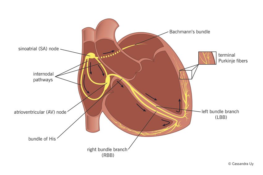
iv

    A real time agorithm based on KNN has been developed for ECG peak
detection, we evaluated the performance with respect to the state of the art and, in
addition, we measured the computational time on Internet of Things (IoT) devices
such as Raspberry Pi 3 and two Android smartphones. This algorithm relies on a
single ECG lead, that means less battery consumption and memory usage, achieving
good results in terms of beat detection accuracy. Furthermore, we demonstrated that
they can operate in real-time on IoT devices which is a real improvement beacuse
there is no need to store the entire sequence of ECG data.

Use Cases
An automated healthcare application [2] allows patients to share information to their
physicians, monitor their health status independently and notify the authorities
rapidly in emergency situations. Any advanced healthcare monitoring system must
be used from both patients and doctors, offline or in real-time, and under all
circumstances. In general, a comprehensive healthcare monitoring system should
support patient self-monitoring, physician offline monitoring through accessing
obtained datasets from various user devices, physician online monitoring and patient
monitoring within healthcare infrastructures such as hospitals and day-care centers.
This analysis leads to the accurate definition of four use cases:

     1. Patient self-monitoring: This use case refers to end-users that would like
        to perform self-monitoring of their medical conditions.

     2. Physician off-line monitoring: This scenario targets doctors that will use
        healthcare products to monitor their patients either at their office or at a
        patients home during a visit. The patients carry the wearable device at home
        and then, after a period of time, return the device to their physician to acquire
        the traces and conduct the diagnosis.

     3. Physician on-line monitoring: This particular use case is an extension of
        the previous one, where the patients use the device over an extended period of
        time and the physician can remotely monitor the acquired vital traces via the
        available cloud services.

     4. Patient monitoring within Healthcare Infrastructures: Being the most
        advanced scenario, this can take place inside an ambulance, hospital or adult
        day-care center whereby the wearable devices, operated by a personal health
        assistant instantly acquire the traces of the patient and enable real-time
        monitoring of the data which are stored to the cloud services.

An example of such application is the HEART platform, that combines wearable
embedded devices, mobile edge devices, and cloud services to provide on-the-spot,
reliable, accurate, and instant monitoring of the heart. Initially, the wearable ECG
goes through a learning phase in order to collect an adequate number of ECG
recordings based on which we will train the pattern matching engine to match the
needs of the particular patient. This is a necessary first step as the evaluation
of and ECG depends on anthropometric data (body height and body weight) on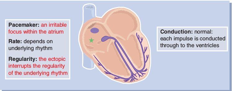
v

Information exchange during the three phases of Learning, Training and Detection, source:[1]

age and sex of a patient. During this phase, the wearable device is continuously
storing the ECG recordings and periodically forwards them to the nearby edge
device. This latter analyzes the received signal and forward it to the cloud services
along with computerized annotations. The authorized physician may view reports,
search traces and examine ECG alerts aggregated on the patient’s health records
remotely after they are synced with the cloud platform. The physician goes through
the annotated recordings and validates or rejects the computerized interpretations
depending on his expert assessment. When an adequate number of normal and
abnormal sessions have been identified by the authorized physician, the system is
ready to enter the training phase. The human-curated annotations are forwarded to
the edge device where the corresponding sessions are extracted from the local storage,
are analyzed to extract a carefully selected set of features. The features of each
session along with the annotations constitute the training vectors for the pattern
matching engine. When the training completes, the wearable device is ready to enter
the detection phase. During the detection phase the signals collected from the ECG
leads are analyzed and the features are extracted using the local processor. The
resulting vector is passed to the pattern matching engine for classification. In case
an abnormal event is detected, the wearable device is in a position to immediately
notify the authorized physician via a short message exchange including only the
alert type. As soon as the patient visits the physician, the complete ECG recordings
are relayed to the nearby edge device. The ECG recordings are finally uploaded
on the cloud platform where they become available to the authorized physician
for examination and assessment. The above described cycle of learning, training
and detecting is repeated periodically to re-evaluate the operation of the pattern
matching of the wearable device and fine-tune its performance. A wearable device
that is used for diagnosing and monitoring heart diseases needs to be capable of
collecting high-quality ECG traces. During the learning phase, the wearable device
is continuously storing the ECG traces on the internal memory. During this offline
monitoring period, the device is expected to store a recorded session of 24 hours.

List of Contributions
   1. QRS KNN algorithm: A new algorithm for heartbeat detection is pre-
vi

       sented, named QRS KNN, that exploits a different feature definition with
       respect to the one explained in [3].This new approach has the advantage
       of requiring a smaller amount of data for training, and resulted in perfor-
       mances(Precision = 0.988 , Recall = 0.923) comparable to the State of the
       Art approaches and lower computational time for both the training and classi-
       fication steps with respect to the implementation of [3].

     2. KNN algorithm: The procedure based on the KNN(K Nearest Neighbors)
        algorithm, described in [3], has been implemented in order to provide a baseline
        for comparison with the QRS KNN. Therefore, the algorithm performance has
        been evaluated and the computational time has been measured.

     3. First-order difference Algorithm: The first-order difference approach
        is a naive algorithm designed to find the local maxima in a generic signal.
        The decision of implementing this approach was taken in order to have a
        comparison between ad-hoc methods for ECG analysis for heartbeat detection
        and a standard signal processing module.

     4. Recurrent Neural Network: The heartbeat detection module aims to
        identify the heartbeats along the ECG tracing. The output of this module is
        then feed to the Arrhythmia classification stage. A Recurrent Neural Network
        has been designed and trained in order to discriminate normal heartbeats to
        the arrhythmic ones. The detected arrhythmic beats are then classified in more
        fine-grained classes, defined by a well-known standard for cardiac algorithm
        evaluation[4].

     5. Comparative Evaluation: A comparative evaluation of the various ap-
        proaches for both heartbeat detection and arrhythmia classification described in
        this study has been provided according to the correctness of the results and the
        computational time. The computational time has been measured executing the
        various algorithms on three different platforms: an Intel®Core™i3-3240 CPU
        @3.40GHz, an Arm Cortex-A53 CPU @2.1GHz and a Qualcomm SnapDragon
        600 CPU @1.9 GHz.

Document Structure
     • Chapter 1: introduction into the cardiological field, and the relationship
       between the ECG signal morphology and the cardiac cycle.

     • Chapter 2: description of the approach followed for the heartbeat detection
       along an ECG record and comparisons with standard solutions.

     • Chapter 3: arrhythmia classification procedure and description of the results.

     • Chapter 4: Conclusions and future work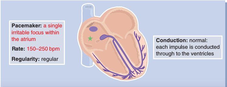
vii

Acknowledgments
Ringrazio i miei genitori che da sempre mi sostengono e Sonia per essermi stata
amorevolmente vicina in questo intenso e meraviglioso anno.
ix
Contents
1 The Heartbeat Cycle: Arrhythmia interpretation on the ECG sig-
nal 1
1.1 The electrical activity of the heart . . . . . . . . . . . . . . . . . . . 1
1.2 Heart conduction system . . . . . . . . . . . . . . . . . . . . . . . . . 1
1.3 Waves and measurements . . . . . . . . . . . . . . . . . . . . . . . . 2
1.3.1 Monitoring leads . . . . . . . . . . . . . . . . . . . . . . . . . 3
1.3.2 Time and voltage measurements . . . . . . . . . . . . . . . . 4
1.3.3 Cardiac cycle from the ECG perspective . . . . . . . . . . . . 4
1.3.4 Artifacts . . . . . . . . . . . . . . . . . . . . . . . . . . . . . . 6
1.3.5 Refractory Periods . . . . . . . . . . . . . . . . . . . . . . . . 6
1.4 Basic Arrhythmias . . . . . . . . . . . . . . . . . . . . . . . . . . . . 7
1.4.1 Sinus Rhythms . . . . . . . . . . . . . . . . . . . . . . . . . . 7
1.4.2 Atrial Rhythms . . . . . . . . . . . . . . . . . . . . . . . . . . 9
1.4.3 Ventricular Rhythms . . . . . . . . . . . . . . . . . . . . . . . 12
1.4.4 Junctional Rhythms . . . . . . . . . . . . . . . . . . . . . . . 14
2 Heartbeat Detection 19
2.1 State of the art . . . . . . . . . . . . . . . . . . . . . . . . . . . . . . 20
2.1.1 Artificial Neural Network . . . . . . . . . . . . . . . . . . . . 20
2.1.2 Convolutional Neural Network . . . . . . . . . . . . . . . . . 21
2.1.3 Hidden Markov Models . . . . . . . . . . . . . . . . . . . . . 22
2.1.4 Support Vector Machine . . . . . . . . . . . . . . . . . . . . . 22
2.1.5 First-Order Difference . . . . . . . . . . . . . . . . . . . . . . 23
2.1.6 Pan Tompkins . . . . . . . . . . . . . . . . . . . . . . . . . . 24
2.2 K Nearest Neighbors approaches . . . . . . . . . . . . . . . . . . . . 24
2.2.1 Signal Preprocessing: Filtering and Squaring Techniques . . . 25
2.2.2 SSK Algorithm . . . . . . . . . . . . . . . . . . . . . . . . . . 26
2.2.2.1 Training . . . . . . . . . . . . . . . . . . . . . . . . 27
2.2.2.2 Model Selection . . . . . . . . . . . . . . . . . . . . 27
2.2.3 QRS KNN Algorithm . . . . . . . . . . . . . . . . . . . . . . 29
2.2.3.1 Training . . . . . . . . . . . . . . . . . . . . . . . . 29
2.2.3.2 Model Selection . . . . . . . . . . . . . . . . . . . . 29
2.3 Evaluation . . . . . . . . . . . . . . . . . . . . . . . . . . . . . . . . . 30
2.3.1 Database . . . . . . . . . . . . . . . . . . . . . . . . . . . . . 31
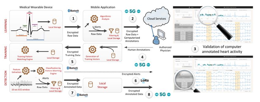
2.3.1.1 Annotations . . . . . . . . . . . . . . . . . . . . . . 31
2.4 Protocol Fine-Tuning . . . . . . . . . . . . . . . . . . . . . . . . . . . 31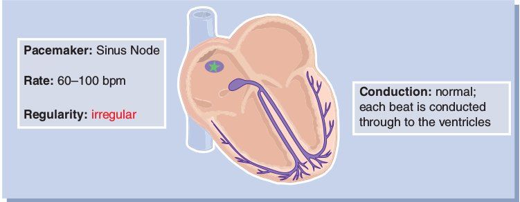
x                                                                                               Contents

          2.4.1   First-Order Difference Algorithm . . . . . . .        .   .   .   .   .   .   .   .   .   32
          2.4.2   SSK Algorithm . . . . . . . . . . . . . . . . .       .   .   .   .   .   .   .   .   .   32
                  2.4.2.1 Model Parameters . . . . . . . . . .          .   .   .   .   .   .   .   .   .   32
          2.4.3 QRS KNN . . . . . . . . . . . . . . . . . . .           .   .   .   .   .   .   .   .   .   32
                  2.4.3.1 Model Parameters . . . . . . . . . .          .   .   .   .   .   .   .   .   .   32
                  2.4.3.2 Window Size . . . . . . . . . . . . .         .   .   .   .   .   .   .   .   .   33
                  2.4.3.3 Channels . . . . . . . . . . . . . . .        .   .   .   .   .   .   .   .   .   33
                  2.4.3.4 Training size . . . . . . . . . . . . .       .   .   .   .   .   .   .   .   .   35
    2.5   Comparative Evaluation . . . . . . . . . . . . . . . .        .   .   .   .   .   .   .   .   .   35
          2.5.1 Results Comparison . . . . . . . . . . . . . .          .   .   .   .   .   .   .   .   .   36
          2.5.2 Computational Time Comparison . . . . . . .             .   .   .   .   .   .   .   .   .   38
    2.6   Critical Issues . . . . . . . . . . . . . . . . . . . . . .   .   .   .   .   .   .   .   .   .   39
          2.6.1 Example 1: First Order Difference Algorithm             .   .   .   .   .   .   .   .   .   39
          2.6.2 Example 2: QRS KNN Algorithm . . . . . .                .   .   .   .   .   .   .   .   .   39

3 Arrhythmia Classification                                                                                 43
  3.1 State of the Art . . . . . . . . . . . . . . . . . . . . . . . . . . . . .                        .   45
      3.1.1 Reservoir Computing and Logistic Regression . . . . . . . .                                 .   45
      3.1.2 Weighted SVM . . . . . . . . . . . . . . . . . . . . . . . . .                              .   45
      3.1.3 Mixture of Experts . . . . . . . . . . . . . . . . . . . . . . .                            .   47
      3.1.4 ECG Morphology and Heartbeat Interval Features . . . . .                                    .   47
  3.2 Recurrent Neural Network . . . . . . . . . . . . . . . . . . . . . . .                            .   48
  3.3 Preprocessing . . . . . . . . . . . . . . . . . . . . . . . . . . . . . .                         .   49
      3.3.1 Input Preparation . . . . . . . . . . . . . . . . . . . . . . .                             .   49
      3.3.2 Dataset Rebalancing . . . . . . . . . . . . . . . . . . . . . .                             .   49
      3.3.3 Standardization . . . . . . . . . . . . . . . . . . . . . . . . .                           .   50
  3.4 Network Structure . . . . . . . . . . . . . . . . . . . . . . . . . . .                           .   50
      3.4.1 Neural Networks Activation Functions . . . . . . . . . . . .                                .   54
  3.5 Training and Validation . . . . . . . . . . . . . . . . . . . . . . . .                           .   56
  3.6 Evaluation . . . . . . . . . . . . . . . . . . . . . . . . . . . . . . . .                        .   56
      3.6.1 Performance Measures . . . . . . . . . . . . . . . . . . . . .                              .   57
      3.6.2 Database Annotations . . . . . . . . . . . . . . . . . . . . .                              .   58
  3.7 Protocol Fine-Tuning . . . . . . . . . . . . . . . . . . . . . . . . . .                          .   58
      3.7.1 Window Size . . . . . . . . . . . . . . . . . . . . . . . . . .                             .   59
      3.7.2 Number of Channels . . . . . . . . . . . . . . . . . . . . . .                              .   60
      3.7.3 Augmentation and Reduction Factors . . . . . . . . . . . .                                  .   61
      3.7.4 Timesteps . . . . . . . . . . . . . . . . . . . . . . . . . . . .                           .   62
      3.7.5 Network Layers . . . . . . . . . . . . . . . . . . . . . . . . .                            .   62
  3.8 Results . . . . . . . . . . . . . . . . . . . . . . . . . . . . . . . . . .                       .   64
      3.8.1 Performance Comparison with State of The Art Algorithms                                     .   65

4 Conclusions and Future Work                                                                               67
1 Chapter 1 The Heartbeat Cycle: Arrhythmia interpretation on the ECG signal The electrical activity of the heart can be monitored by the ECG tracing, while the mechanical activity is evaluated by assessing pulses and blood pressure [5]. An ECG record is designed to give a graphic display of the electrical activity of the heart. The pattern displayed on the ECG is called rhythm. Therefore, the word arrhythmia refers to an abnormal heart rhythm. 1.1 The electrical activity of the heart At the start of the cycle, when the heart is in a resting state, positive and negative electrical charges are balanced. This is called the polarized state, where no electrical flow is generated. A difference of potential between the inside of the heart and the outside is needed for the organ in order to receive the stimulus to start beating. When the charges inside and outside the earth trade places, the electricity flows in a wave-like motion throughout the heart. This wave is called depolarization, i.e. the process of the electrical discharge and flow of electrical activity. The process that follows the depolarization, which brings the heart ot the initial state, is called repolarization. 1.2 Heart conduction system The electrical cells in the heart are all arranged in a system of pathways, called the conduction system. The study of this system is an essential part for the arrhythmia interpretation purpose. Normally, the electrical originates in the Sinoatrial(SA) node and travels to the ventricles by way of the AV node; 1.1 after leaving it, the impulses go through the Bundle of His to reach the right and left bundle branches, located within the right and left ventricles. At the terminal ends of the bundle branches, small fibers distribute the electrical impulses to muscle cells to stimulate contraction. These fibers are called Purkinje fibers.
2 1. The Heartbeat Cycle: Arrhythmia interpretation on the ECG signal
Figure 1.1. Electrical Conduction through the Heart, source:[5]
Each site has its own rate, called inherent rate at which it initiates impulses.
The SA node, in normal conditions, has the greatest inherent rate; for this it is the
normal pacemaker of the heart. If, however, a site becomes irritable and begins to
discharge impulses at a faster than normal rate, it can override the SA node and
take over the pacemaking function for the heart. This mechanism of an irritable
site speeding up and taking over as pacemaker is called irritability. It is usually
an undesirable occurrence, since it overrides the normal pacemaker and causes the
heart to beat faster than it otherwise would. Something very different happens if
the normal pacemaker slows down for some reason. If the SA node drops below
its inherent rate, or if it fails entirely, the site with the next highest inherent rate
will usually take over the pacemaking role. The next highest site is within the AV
junction , so that site would become the pacemaker if the SA node should fail. This
mechanism is called escape and is a safety feature that is built into the heart to
protect it in case the normal fails.
1.3 Waves and measurements
The electrical patterns of the heart can be picked up from the surface of the skin
by attaching an electrode and connecting it to a machine that will display the
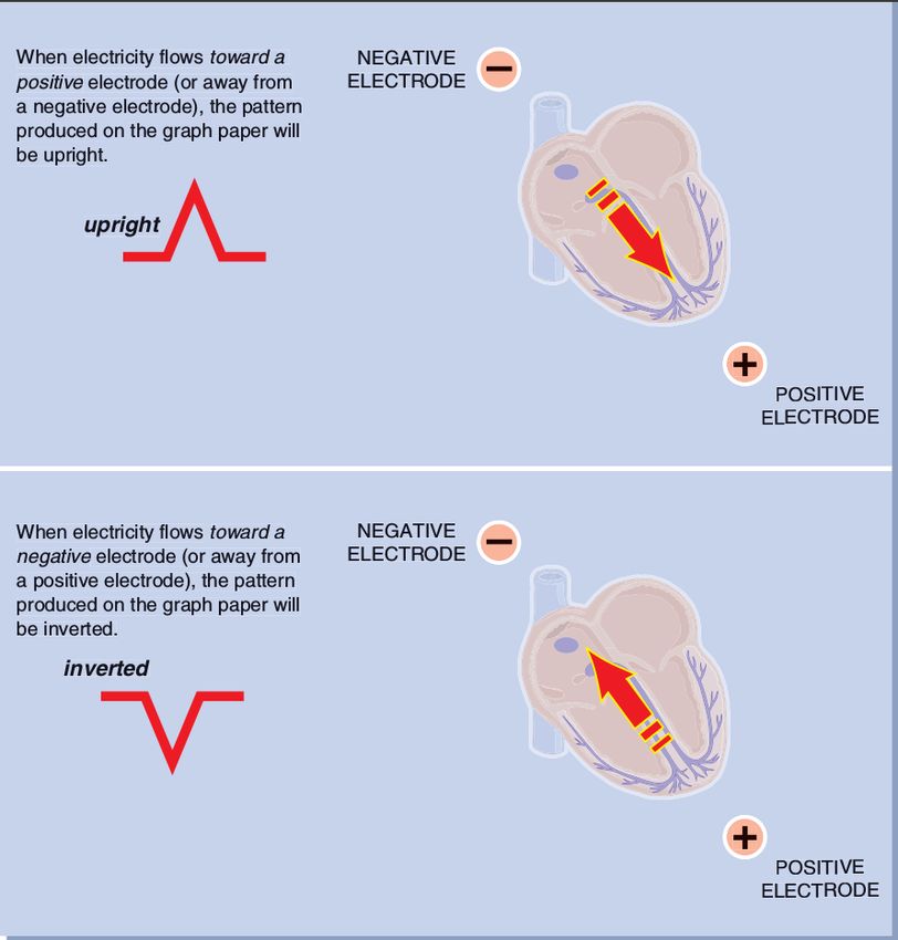
electrical activity on a graph paper. There is a basic rule regarding the flow of
electricity through the heart and out of the electrodes: if the electricity flows toward
the positive electrode, the patterns produced on the graph paper will be upright.
Conversely, if the electricity flows away from the positive electrode or passes through
the negative one, the pattern will be a downward deflection. 1.21.3 Waves and measurements 3
Figure 1.2. Rule of electrical flow, source:[5]
1.3.1 Monitoring leads
The positioning of an electrode for monitoring the ECG allows to see a single
view of the heart’s electrical pattern. Each view of the heart is called lead. For
sophisticated ECG interpretation, many leads are inspected to visualize the entire
heart, however for basic interpretations of arrhythmia only one single lead can be
considered sufficient. Single lead that give good pictures of the basic waves are called
monitoring leads beacuse they are used to monitor patterns such as arrhythmia. The
first widely used monitoring lead was Lead II, but now it is common to use other
leads as well, especially variations of the chest leads(M CL1 for instance). Figure
1.3 shows the placement of electrodes to monitor Lead II. Note that the positive
electrode is at the apex of the heart, and the negative electrode is below the right
clavicle.The third electrode is a ground electrode and does not measure electrical
flow in this lead. A widely used configuration of electrodes is one composed of 10
electrodes: one of the electrodes is positioned on the left arm (LA), on on the right
arm (RA), one on the left leg (LL), one on the right leg (LL) and six on the chest(V1
to V6), allowing a formation of 12 leads[6]. The 10 electrodes (12 lead) configuration
can be seen in 1.44 1. The Heartbeat Cycle: Arrhythmia interpretation on the ECG signal
Figure 1.3. Electrode Placement for Monitoring Lead II, , source:[5]
Figure 1.4. Typical 10 electrodes configuration, source:[6]
1.3.2 Time and voltage measurements
It is the strength of the current, or its voltage, that will determine the magnitude of
the deflection. Therefore, the height of the deflection will indicate the amplitude of
the electrical charge that produced the deflection. The second, and more important
thing that the graph paper can provide is the determination of time. The vertical
lines in the graph paper can tell how much time it took to the electrical current
within the heart to travel from one area to another. This information is one of the
most important for identifying an arrhythmia.
1.3.3 Cardiac cycle from the ECG perspective
The heart has four chambers: the upper two are the atria and the lower two are
the ventricles. Atria and ventricles both operates as a single unit. In the normal
heart, blood enters both atria simultaneously and then is forced into both ventricles
simultaneously as the atria contract. All of this is coordinated so that the atria fill
while the ventricles contract and viceversa. During each phase of the cardiac cycle, a
distinct pattern is produced on the ECG graph paper. By learning to recognize these
wave patterns and the cardiac activity they represent, we can study the relationships1.3 Waves and measurements 5
between the different areas of the heart and begin to understand what is taking
place within the heart at any given time.
In the ECG, each of the heartbeat phases is displayed by a specific wave pattern.
A single cardiac cycle is expected to produce one heartbeat. In labeling the activity
on the graph paper, the deflection above or below the median (a.k.a. isoelectric) line
are called waves. In a single cardiac cycle there are five prominent waves, and each
is labeled with a letter. In Figure 1.5 is it possible to determine the P, Q, R, S and
T waves. An interval refers to the area between waves, and a segment identifies a
Figure 1.5. The ECG complex
straight line or area of electrical inactivity between waves.
The first identifiable wave of the cardiac cycle is the P wave. The P wave
starts with the first deflection from the isoelectric line. It is indicative of atrial
depolarization.
As the impulse leaves the atria and travels to the AV node, it encounters a slight
delay. The tissues of the node do not conduct impulses as fast as other cardiac
electrical tissues. This means that the wave of depolarization will take a longer time
to get through the AV node than it would be in other parts of the heart. On the
ECG, this is translated into a short period of electrical inactivity called the PR
segment.
The subsequent wave is the QRS complex. The ventricular depolarization is
shown by the ECG by a large complex of three waves: the Q, the R, and the S.
This wave is significantly larger than the P wave beacuse ventricular depolarization
involves a greater muscle mass than atrial depolarization. The Q wave is defined as
the first negative deflection following the P wave but before the R wave. The Q wave6 1. The Heartbeat Cycle: Arrhythmia interpretation on the ECG signal
flows immediately into the R wave, which is the first positive deflection following
the P wave.
Next comes the S wave, which is defined as the second negative deflection
following the P wave, or the first negative deflection following the R wave.
After the ventricles depolarize, they begin their repolarization phase, which results
in another wave in the ECG. The T wave is indicative of ventricular repolarization.
The atria also repolarize, but this event is not significant enough to show up in the
ECG.
Between the S and the T wave is a section called the ST segment. The ST
segment is the flat, isoelectric section of the ECG between the end of the S wave and
the beginning of the T wave. It represents the interval between ventricular depolari-
sation and repolarisation. The most important cause of ST segment abnormality
(elevation or depression) is myocardial ischaemia / infarction.
1.3.4 Artifacts
The complexes on an ECG tracing are created by electrical activity within the heart.
But it is possible for things other than cardiac activity to interfere with the tracing
under analysis. Some common causes of interference, or, artifact are:
• Muscle tremors
• Patient movement
• Loose electrodes
• The effect of other electrical equipment in the room.
All these artifacts may interfere with the arrhythmia interpretation, because they
may cause deflections on the signal.
1.3.5 Refractory Periods
Since depolarization takes place when the electrical charges begin their wave of
movement by exchanging places across the cell membrane, it would follow that this
process cannot take place unless the charges are in their original position. This
means that the cell cannot depolarize until the repolarization process is complete.
When the charges are depolarized and have not yet returned to their polarized state,
the cell is said to be electrically refractory because it cannot yet accept another
impulse.
On the ECG, the refractory period of the ventricles is when they are depolarizing
or repolarizing. Thus, the QRS and the T wave on the EKG would be considered
the refractory period of the cardiac cycle, since it signifies a period when the heart
would be unable to respond to an impulse. Sometimes an electrical impulse will try
to discharge the cell before repolarization is fully complete. In most cases nothing
will happen because the cells are not back to their original position and therefore1.4 Basic Arrhythmias 7
cannot depolarize. But once in a while, if the stimulus is strong enough, an impulse
might find several of the charges in the right position and thus discharge them before
the rest of the cell is ready. This results in abnormal depolarization and hence is an
undesirable occurrence. Thus, there is a small part of the refractory period that is
not absolutely refractory. This small section is called the relative refractory period
because some of the charges are polarized and thus can be depolarized if the impulse
is strong enough.
1.4 Basic Arrhythmias
Arrhythmia analysis is a quite complex task since not only does every person on
earth have his or her own individual ECG, distinct from all others, but one person’s
ECG can look very different from one moment to the next. It is inadequate to
memorize some of the most common ECG patterns and trying to recognize them in
the future. This type of ECG analysis is called pattern recognition and is a common
but accidental way to approach arrhythmias. A much more reliable way to approach
an EKG tracing is to take it apart, wave by wave, and interpret exactly what’s
happening within the heart.
Arrhythmias can be categorized into groups according to which pacemaker site
initiates the rhythm. The most common sites, and thus the major categories of
arrhythmias, are:
• Sinus
• Atrial
• Junctional
• Ventricular
The most common cardiac rhythm is sinus in origin, because the sinus(SA) node is
the usual pacemaker of the heart (Section 1.2). Therefore, a normal, healthy heart
would be in Normal Sinus Rhythm (NSR) because the rhythm originated in
the SA node.
1.4.1 Sinus Rhythms
This category comprehends the rhythms originating in the Sinus node (SA) (Section
1.2). This group includes:
• Normal Sinus Rhythm
• Sinus Bradychardia
• Sinus Tachycardia
• Sinus Arrhythmia8 1. The Heartbeat Cycle: Arrhythmia interpretation on the ECG signal
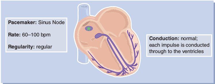
Technically speaking, the Normal Sinus Rhythm is not an arrhythmia beacause it
is a normal, rhythmic pattern. In a Normal Sinus Rhythm 1.6 the pacemaker impulse
originates in the sinus node and travels through the normal conduction pathways
within normal time frames. The P waves will be uniform, and since conduction
is normal, one P wave will be in front of every QRS complex. Since the SA node
Figure 1.6. Mechanism of the Normal Sinus Rhythm, source:[5]
inherently fires at a rate of 60-100 times per minute, a Normal Sinus Rhythm must,
by definition, fall within this rate range.
If a rhythm has all the characteristics of a NSR except fot the rate, that is lower
than 60 bpm, it is called a bradychardia(Fig. 1.7), meaning slow heart.
Figure 1.7. Mechanism of Sinus Bradychardia, source:[5]
The same thing is true for a rhythm that fits all of the rules for NSR except
that the rate is too fast. When the heart beats too fast, it is called tachycardia,
meaning fast heart. So a rhythm that originates in the sinus node and fits all rules
for NSR except that the rate is too fast will be called Sinus Tachycardia(Fig. 1.8).
Figure 1.8. Mechanism of Sinus Tachychardia, source:[5]1.4 Basic Arrhythmias 9
Finally, The Sinus Arrhythmia(Fig.1.9) is characterized by a pattern that
would normally be considered NSR, except that the rate changes with the patient’s
respirations. When the patient breathes in, the rate increases, and when he or she
breathes out, the rate slows. This causes the R-R interval to be irregular across the
strip. The result is a pattern with an upright P wave in front of every QRS complex,
a normal and constant PRI, a normal QRS complex, but an irregular R-R interval.
The difference between NSR and Sinus Arrhythmia is that NSR is regular and Sinus
Arrhythmia is irregular.
Figure 1.9. Mechanism of Sinus Arrhythmia, source:[5]
1.4.2 Atrial Rhythms
Sometimes the sinus node loses its pacemaking role, and this function is taken over
by another site along the conductive system. The site with the fastest inherent rate
usually controls the pacemaking function, as explained in Section 1.2. Since the
atria have the next highest rate after the SA node, it is common for the atria to
take over from the SA node. Rhythms that originate in the atria are called atrial
arrhythmias. Atrial arrhythmias are caused when the atrial rate becomes faster
than the sinus rate, and an impulse from somewhere along the atrial conduction
pathways is able to override the SA node and stimulate depolarization. As with a
sinus rhythm, an impulse that originates in the atria will travel through the atria
to the AV junction anf then through the ventricular conduction pathways to the
Purkinje fibers. The only difference is in the atria, where the conduction will be a
little slower and rougher than it is with sinus rhythms.
Since atrial depolarization is is seen on the ECG as a P wave, it is expected
to be of unusual shape. It can be flattened, notched, peaked, sawtoothed or even
diphasic( meaning that it goes first above the isoelectric line and then dips below it.)
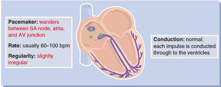
The first presented atrial arrhythmia is called Wandering Pacemaker (Figure
1.10). Wandering Pacemaker is caused when the pacemaker role switches from beat
to beat from the SA node to the atria and back again. The result is a rhythm
made up of interspersed sinus and atrial beats. The sinus beats are preceded by
nice, rounded P waves, but the P wave changes as the pacemaker drops to the atria.
The P waves of the atrial beats are not consistent and can be any variety of atrial
configuration (e.g., flattened, notched, diphasic). In Wandering Pacemaker, the
rhythm is usually slightly irregular.10 1. The Heartbeat Cycle: Arrhythmia interpretation on the ECG signal
Figure 1.10. Mechanism of Wandering Pacemaker, source:[5]
When a single beat arises from an ectopic focus (a site outside of the SA node)
within the conduction system, that beat is called ectopic beat. When an ectopic
beat originates in the atria, it is called and atrial ectopic. An ectopic beat arises
when a site somewhere along the conduction system becomes irritable and overrides
the SA node for a single beat.
An atrial ectopic that is caused by irritability is called a Premature Atrial
Complex(PAC)(Figure 1.11). A PAC is an ectopic beat that comes early in the
cardiac cycle and originates in the atria.
Figure 1.11. Mechanism of Premature Atrial Complex, source:[5]
A rhythm with PACs will be irregular beacuse the ectopics come permaturely
and interrupt the underlying rhythm. Because PACs originate in the atria, they will
have a characteristic atrial P wave that differs in morphology from the sinus P wave.
It is also possible for a single focus in the atria to become so irritable that it begins
to fire very regularly and thus overrides the SA node for the entire rhythm. This
arrhythmia is called Atrial Tachycardia (AT) (Figure 1.12) Atrial Tachycardia
Figure 1.12. Mechanism of Atrial Tachycardia, source:[5]1.4 Basic Arrhythmias 11
will have all of the charachteristics of a PAC, except that is an entire rhythm instead
of a single beat. All of the P waves in AT will have an atrial configuration. Atrial
Tachycardia is a charachteristically very regular arrhythmia. It is usually very rapid,
with a rate range between 150 and 250 bpm.
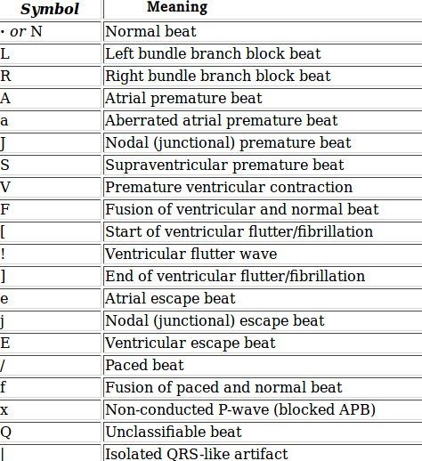
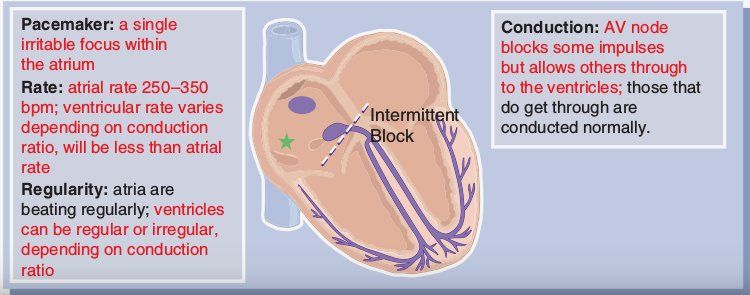
When the atria become so irritable that they fire faster than 250 bpm, they are
said to be fluttering.This rhythm is called Atrial Flutter. In this case the atrial
rate is usually in the range of 250-350 bpm.
Figure 1.13. Mechanism of Atrial Flutter, source:[5]
The problem with a heart rate this rapid is that the ventricles don’t have
enough time to fill with blood between each beat. The result is that the ventricles
will continue to pump but they won’t be ejecting adequate blood volume to meet
body needs. The heart has a built-in protective mechanism to prevent this from
happening: the AV node. The AV node is responsible for preventing excess impulses
from reaching the ventricles. This blocking action allow the ventricles to have time
to fill with blood before they have to contract. This will be seen on the ECG as a
very rapid series of P waves(Flutter Waves), but not every one followed by a QRS
complex.
The last atrial arrhythmia in this study is the Atrial Fibrillation(Figure 1.14)
This rhythm result when the atria become so irritable that they are no longer
beating but are merely quivering ineffectively. This quivering ineffectively is called
fibrillation. On the ECG tracing it is seen as a series of indescirnible waves along
Figure 1.14. Mechanism of Atrial Fibrillation, source:[5]
the isoelectric line. In Atrial Fibrillation there are no discirnible P waves. The
fibrillatory waves characteristic of Atrial fibrillation are called f waves. The rhythm
is grossly irregular because the fibrillatory waves are conducted in a very chaotic
way.12 1. The Heartbeat Cycle: Arrhythmia interpretation on the ECG signal
1.4.3 Ventricular Rhythms
Ventricular Arrhythmias are very serious for several reasons. First, the heart was
intended to depolarize from the top down. The atria were meant to contract before
the ventricles in order to pump blood effectively. When an impulse originates in
the ventricles, the process is reversed, and the heart’s efficiency is greatly reduced.
Furthermore, since the ventricles are the lowest site in the conduction system, there
are no more fail-safe mechanisms to backup a ventricular arrhythmia. In this section
five ventricular arrhythmias are presented:
• Premature Ventricular Contraction
• Ventricular Tachychardia
• Ventricular Fibrillation
• Idiovenrticular Rhythm
• Asystole
The Premature Ventricular Complex(PVC)(Figure 1.15)is not a rhythm
but instead a single ectopic beat originating from an irritable ventricular focus. For
this reason, the complex will come earlier than expected on the cardiac cycle and will
interrupt the regularity of the underlying rhythm. Because PVCs originate in the
ventricles, the QRS will be wider than normal. But a second feature of a ventricular
focus is that there is no P wave preceding the QRS complex. One of the things that
Figure 1.15. Mechanism of Premature Ventricular Contraction, source:[5]
gives a PVC a bizarre appearance, in addition to the width of the QRS complex, is
the tendency for PVCs to produce a T wave that extends in the opposite direction
of the QRS complex. Another frequent feature that may be helpful in identifying a
PVC is the compensatory pause that usually follows a ventricular ectopic.
A compensatory pause is created when a PVC comes early, but since it doesn’t
conduct the impulse retrograde through the AV node, the atria are not depolarized.
This leaves the sinus node undisturbed and able to discharge again at its next
expected time. The result is that the distance between the complex preceding the
PVC and the complex following the PVC is exactly twice the distance of one R-R
interval.1.4 Basic Arrhythmias 13
Another configuration possibility is that the PVC be followed by no pause what-
soever. This occurs when the PVC squeezes itself in between two regular complexes
and does not disturb the regular pattern of the sinus node. This phenomenon is
called an interpolated PVC, because the PVC inserts itself between two regular
beats
If the myocardium is extremely irritable, the ventricular focus could speed up and
override higher pacemaker sites. This would create what is essentially a sustained
run of PVCs. This rhythm is called Ventricular Tachychardia(VT)(Figure 1.16)
In ventricular tachychardia you will see a succession of PVCs across the strip at a
Figure 1.16. Mechanism of Ventricular Tachychardia, source:[5]
rate of about 150-250 bpm. This arrhythmia usually has a very uniform appearance,
even though the R-R interval may be slightly irregular. It is possible for VT to
occur at slower rates, but when it does, it is qualified by calling it a slow VT. All
the description related to PVCs apply to VT.
In extremely severe cases of ventricular irritability, the electrical foci in the
ventricles can begin fibrillating. This means that many foci are firing in a chaotic,
ineffective manner, and that the heart muscle is unable to contract in response.
Ventricular Fibrillation(Figure 1.17) is a lethal arrhythmia, since the rhythm is
very chaotic and ineffective. Ventricular Fibrillation (VF) is probably the easiest of
Figure 1.17. Mechanism of Ventricular Fibrillation, source:[5]
all the arrhythmias to recognize. This is because there are no discernible complexes
or intervals and the entire rhythm consists of chaotic, irregular activity. VF has no
measurable waves or complexes.
There are two ways a ventricular focus can assume control of the heart. One is
irritability and the other is escape(see Section 1.2). A ventricular escape rhythm
is one that takes over pacemaking in the absence of a higher focus and depolarizes14 1. The Heartbeat Cycle: Arrhythmia interpretation on the ECG signal
the heart of the inherent rate of the ventricles, which is 20-40 bpm. This rhythm
is called Idioventricular Rhythm(Figure 1.18). It is not possible to see P waves
in an Idioventricular Rhythm, since the escape mechanism would take over only if
the atrial pacemaker sites had failed. Idioventricular Rhythm is initiated by the
Figure 1.18. Mechanism of Idioventricular Rhythm, source:[5]
very last possible fail-safe mechanism within the heart. When the rhythm is in its
terminal stages, that is, as the patient is dying, the complexes can lose some of their
form and be quite irregular. In this stage, the arrhythmia is said to be agonal, or
a dying heart. The word agonal is used to describe a terminal, lethal arrhythmia,
especially when it has stopped beating in a reliable pattern. Idioventricular Rhythm
is an agonal rhythm, especially when the rate drops below 20 bpm and the pattern
loses its uniformity.
The last stage of a dying heart is when all electrical activity ceases. This results
in a straight line on the ECG, an arrhythmia called Asystole Asystole is a lethal
Figure 1.19. Mechanism of Idioventricular Rhythm, source:[5]
arrhythmia that is very resistant to resuscitation effort
1.4.4 Junctional Rhythms
The AV junction consists of the AV node and the Bundle of His(see Section 1.2).
This unique part of the conduction system is responsible for conducting impulses
from the SA node down the conduction pathways to the ventricles. The body of
the AV node is responsible for delaying each impulse just long enough to give the
ventricles time to fill before contracting. The lower region of the AV junction
houses the pacemaking cells that initiate the group of arrhythmias called junctional
rhythms.1.4 Basic Arrhythmias 15
When electrical impulses originate in the AV junction, the heart is depolarized in
a somewhat unusual fashion: with the pacemaker located in the middle of the heart,
the impulses spread in two directions simultaneously(see Figure 1.20). Recalling
from Section 1.3.1, electrode positions for Lead II place the negative electrode
above the right atria and the positive electrode below the ventricle. In the normal
Figure 1.20. Electrical Flow in Junctional Arrhythmias, source:[5]
heart, the major thrust of electrical flow is toward the ventricles (and toward the
the positive electrode in Lead II), thus producing an upright QRS complex. In a
junctional rhythm, the ventricles are depolarized by an impulse travelling down the
conduction system toward the positive electrode; thus the QRS complex is upright.
But, at the same time, the impulse can spread upward through the atria toward the
negative electrode. When the atria are depolarized in this backward fashion, it is
called retrograde conduction because the electrical impulse travels in the opposite
direction it usually takes. Thus, the atrial activity will produce a negative deflection
on the ECG. In other words, the P wave of an AV junctional arrhythmia should
be inverted beacuse it was produced by an impulse travelling toward the negative
electrode.
In junctional arrhythmias, the P wave does not always have to precede the QRS
complex beacause it is possible for the ventricles to be depolarized before the atria,
if the force reach them first. If they both depolarize simultaneously the P wave will
be hidden within the QRS complex.
The junctional pacemaker site can produce a variety of arrhythmias, depending
on the mechanism employed. Four basic mechanisms common to the AV junction
will be discussed:
• Premature Junctional Complex
• Junctional Escape Rhythm
• Accelarated Junctional Rhythm
• Junctional Tachycardia
The Premature Junctional Complex or PJC (Figure 1.21), is not an entire
rhythm; it is a single ectopic beat. A PJC is similar in many ways to a Premature
Atrial Contraction(PAC)(see Section 1.4.2). In the case of PJC, the irritable focus
comes from the AV junction to stimulate an early cardiac cycle, which interrupts
the underlying rhythm for a single beat. The P wave of a PJC is inverted as for the
others junctional arrhythmias.16 1. The Heartbeat Cycle: Arrhythmia interpretation on the ECG signal
Figure 1.21. Mechanism of Premature Junctional Complex, source:[5]
A Junctional Escape Rhythm (Figure 1.22) is expected to have a rate of
40-60 bpm since this is the inherent rate of the AV junction.
Figure 1.22. Mechanism of Junctional Escape Rhythm, source:[5]
A junctional escape rhythm has all the characteristics previously described of a
junctional arrhythmia. Such rhythm us a fail-safe mechanism rather than an irritable
arrhythmia(see Section 1.2). However, the AV junction is capable of irritability
and is known to produce an irritable arrhythmia called Junctional Tachycardia.
This rhythm occurs when the junction initiates impulses at a rate faster than its
inherent rate of 40-60 bpm, thus overriding the SA node. Junctional Tachycardia is
usually divided in two categories, depending on how fast the irritable site is firing.
If the junciton is firing between 60 and 100 bpm, the arrhythmia is termed an
Accelarated Junctional Rhythm(Figure 1.23 ) When the rate exceeds 100 bpm,
Figure 1.23. Mechanism of Accelerated Junctional Rhythm, source:[5]
the rhythm is considered a Junctional Tachycardia (Figure 1.24 )
Junctional Tachycardia can be as fast as 180 bpm, but at this rapid rate, it is
extremely difficult to identify positively since P waves are superimposed on preceding
T waves.1.4 Basic Arrhythmias 17
Figure 1.24. Mechanism of Junctional Tachycardia, source:[5]
The only difference appreciable on the ECG signal among Junctional Escape
Rhythm, Accelarated Junctional Rhythm and Junctional Tachycardia is the rate.
The rates are listed in table 1.1 :
Rhythm Rate(bpm)
Junctional Escape 40-60
Accelerated Junctional 60-100
Junctional Tachycardia 100-180
Table 1.1. Rates of Junctional Rhythms, source:[5]19
Chapter 2
Heartbeat Detection
The first stage of an arrhythmia detection system consists in the extraction of
heartbeats along the ECG signal. In the following chapter it is described the
Heartbeat Detection module, aimed to locate a sequence of heartbeats inside a
raw ECG signal.
The heartbeat, as observed in the ECG tracing, is composed by three waves
(Section 1.3.3): the P, QRS and the T wave. The most prominent in terms of
amplitude is the QRS wave and therefore it is the easiest to detect. Hence, the
heartbeat detection problem is equivalent to the QRS detection.
The QRS detection problem, on its standard formulation, takes as input an ECG
sample and computes whether it resides in a QRS wave.
QRS detection is difficult, because the beat morphology varies along the time,
and different sources of noise can be present[7]. Noise sources include muscle noise,
artifacts (Section 1.3.4) due to electrode motion, power-line interference, baseline
wander, and T waves with high-frequency characteristics similar to QRS complexes.[9]
Most QRS detection algorithms have two differentiated stages: preprocessing
and decision [8]. In preprocessing stage different techniques are applied to the signal,
such as linear and non-linear filtering or smoothing to attenuate P and T waves
as well as noise. In decision stage the most important task is the determination of
thresholds and in some cases the use of techniques to discriminate T waves. Some
algorithms include another decision stage to reduce false positives.
Once the QRS waves have been detected, it is possible to solve the more specific
R Peak detection problem: The R peak is the sample of maximal amplitude
inside the QRS wave. From the locations of the R peaks in the ECG tracing it
is possible to extract the complete sequence of heartbeats, useful for arrhythmia
analysis purposes.
In this work, the R peak detection problem is formalized as a Machine Learn-
ing task. This is possible when dealing with databases annotated by expert
cardiologists: a learning algorithm is trained on the labeled data in order to ex-
tract useful knowledge to be applicable to real world data. This scenario is the20 2. Heartbeat Detection
standard Supervised Learning framework. In this study, two Supervised learning
approaches based on the KNN algorithm have been implemented and evaluated in
terms of quality of the results and computational time measured on different IoT
platforms. Another algorithm has been implemented in order to provide a more
complete comparison: the First-Order difference algorithm is a naive algorithm
designed to find the local maxima in a generic signal. The decision of considering
this approach was taken in order to have a comparison between ad-hoc methods for
ECG analysis for heartbeat detection and a standard signal processing module.
In Section 2.1 a selection of the most representative state of the art algorithms for
R Peak detection, including the aforementioned one, have been described. In Section
2.2 it is possible to find a description of the procedures based on the KNN algorithm
implemented in this study in order to solve the heartbeat detection problem. In
Section 2.3 we define the assumptions considered for evaluating the procedures
in terms of correctness of the results and computational time. In Section 2.4 we
report all the combinations of parameters studied and the obtained score, in order
to select the best ones for each beat detection algorithm. In Section 2.5 a complete
comparison between the implemented approaches is presented.
2.1 State of the art
2.1.1 Artificial Neural Network
The approach described in [10] consists in a novel QRS complex detector using 3-
layer artificial feedforward back propagation neural network. The training
method is Levenberg-Marquardt back propagation. After baseline drifts elimi-
nation and lowpass filtering, each sample in ECG signal is extractedand then
given as input to the neural network. The algorithm is tested with the MIT-BIH
Arrhythmia Database records and the accuracy is 99.5%. Baseline drifts elimination
is done using two median filters (200-ms and 600-ms). The 200-ms median filter
is for removing QRS-complexes and P-waves while the 600-ms median filter is for
removing the T-waves. By subtracting the filtered signal from the original signal,
the baseline drifts and artifacts are removed. In order to reduce the size of the
input of the neural network, features of each sample are firstly extracted. This is
accomplished by a function called Features Extractor whose inputs are the ECG
signal and the sample identifier, n . The output of Features Extractor is a matrix of
three rows of values, which are shown below.
1. The average amplitude of the samples from n -16 to n +16
2. The average of derivatives of samples before n, which are n − 1, n − 2, n − 5,
n − 10, n − 20, n − 50, n − 100.
3. The average of derivatives of samples after n , which are n + 1, n + 2, n + 5,
n + 10, n + 20, n + 50, n + 100.
The output of the ANN is just a number which ranges between -1 and 1. By using a
Sign function, the positive output values of ANN means the corresponding samples2.1 State of the art 21
are determined to be R-peak and the negative output values means the corresponding
samples are determined not R-peak.
In the conclusive section of the paper is reported that the accuracy obtained
on the recordings of MIT-BIH arrhythmia database used as test is 99.5%, but it
is not clear what criterion has been followed for the dataset partition in training
and test set. Furthermore, the accuracy measure is not relevant in this context,
because of the Accuracy paradox.1 Precision and recall measures are more reliable
in classification problems in which one or more classes are dominant with respect to
others.
2.1.2 Convolutional Neural Network
In the paper [11] it is presented a QRS detection algorithm based on pattern
recognition as well as a new approach to ECG baseline wander removal and signal
normalization. Each point of the zero-centred and normalized ECG signal is a
QRS candidate, while a 1-D CNN classifier serves as a decision rule. Positive
outputs from the CNN are clustered to form final QRS detections. The data is
obtained from the 44 non-pacemaker recordings of the MIT-BIH arrhythmia
database. Classifier was trained on 22 recordings and the remaining ones are used
for performance evaluation. The preprocessing step is conducted solely to ensure the
data is zero-centred and normalized for the classifier training and prediction step.
The idea is to have a well extracted ECG morphology, with as little information loss
as possible. Every point of the signal was described by a sample of 145 neighbouring
points, resulting in a total of 14296832 data samples. Each data sample is labelled
positive if the candidate point is inside a Âś40ms distance of an original positive
beat annotation. The proposed CNN architecture besides a 1-D input layer, consists
of two convolutional layers with a max-pooling layer between them , two fully-
connected layers and a softmax classification layer. All convolutional and fully-
connected layers have a dropout probability of 0.5 to reduce overfitting on training
data and make the trained model less sensitive to partial deformations of ECG
morphology. Stochastic gradient descent with 0.9 momentum and an initial learning
rate of 0.005 was used to train the network. Mini-batch size was 128 samples, and
the training was limited to 3 epochs. After the classification step, they performed a
hierarchical group-average agglomerative clustering upon all CNN decisions
of a single recording, with clustering criterion being the temporal euclidean distance.
Final QRS detection is the mean of all CNN detections within the same cluster. To
determine whether a detection is a true positive (TP), a Âś75ms tolerance window
is used. This method achieves a sensitivity of 99.81% and 99.93% positive predictive
value, which is comparable with most state-of-the-art solutions.
1
The accuracy paradox is the paradoxical finding that accuracy is not a good metric for predictive
models when classifying in predictive analytics. This is because a simple model may have a high
level of accuracy but be too crude to be useful. For example, if the incidence of category A is
dominant, being found in 99% of cases, then predicting that every case is category A will have an
accuracy of 99%. Precision and recall are better measures in such cases22 2. Heartbeat Detection
2.1.3 Hidden Markov Models
An HMM [12] is a statistical model used to characterize signal dynamics as a function
of time. A typical HMM is composed of n hidden states and the set of parameters
λ = (A, B, π), where:
1. A = aij is the matrix of state transition probability distribution from state i
to j.
2. B = bj (k) is the observation symbol probability distribution in state j.
3. π = πi is the initial state distribution.
A training stage is performed to obtain the set of parameters λ in order to maximize
P (Otrain |λ), the probability that an observation sequence Otrain = O1 , O2 ..., OT ,
taken from the analyzed system, is generated by the model. In the work explained
in [13], an automatic QRS complex detector based on continuous density hid-
den Markov models (HMM) is proposed. HMM were trained using univariate
observation sequences taken either from QRS complexes or their derivatives. The
detection approach is based on the log-likelihood comparison of the observation
sequence with a fixed threshold. A sliding window was used to obtain the observation
sequence to be evaluated by the model. The threshold was optimized by receiver
operating characteristic curves. Sensitivity (Sen), specificity (Spc) and F 1 score
were used to evaluate the detection performance. The approach was validated using
ECG recordings from the MIT-BIH Arrhythmia database. A 6-fold cross-validation
shows that the best detection performance was achieved with 2 states HMM trained
with QRS complexes sequences (Sen = 0.668, Spc = 0.360 and F 1 = 0.309).
2.1.4 Support Vector Machine
The paper [14] presents an algorithm for QRS complex detection based of support
vector machine (SVM). The proposed algorithm is evaluated on annotated standard
databases such as MIT- BIH Arrhythmia database. The procedure of preliminary
processing of a signal is used as the signal contains different noise and artifacts:a
low pass filter with a cut-off frequency of 13 Hz and high pass filter with a cut- off
frequency of 9 Hz are used, as well as the function of the moving average with a
5 measurements window sizes. Informative feature as rise speed of a signal is
chosen, because QRS complex possesses the greatest climb rate. This informative
feature is implemented as follows: an array of the values of the slope of the tangent
to each point of the filtered and squared ECG signal. After that SVM classification
function is applied to the received selection. Informative feature as correlation
forms of QRS-complexes are chosen, because QRS-complex possesses a specific
form. This informative feature is implemented as follows: Firstly, test pulse is created
based on 1000 QRS-complexes with the R-peak in the middle lasting 51 counting
(141.67 ms), which occurs after their averaging, for this procedure the signal N.100
is used. Secondly, an array of correlation coefficients forms of QRS-complexes in
a moving window is created. After that SVM classification function is applied to
the received selection. For train recording signals No100, No104, No214, No200,
No205 are used. The training set consists of 30,000 values for each of the signs.2.1 State of the art 23
The function of classification was calculated for each informative feature separately.
Signals from MIT-BIH database with 30 min of duration are used for testing. After
testing, a train of 1’s is obtained at the output of SVM classifier. Then this train of
1’s is picked and by using their duration, average pulse duration of 1’s is evaluated.
Those trains of 1’s, whose duration turns out to be more than the average pulse
duration are detected as QRS-complex and the others are discarded. The QRS
detector obtained a sensitivity Se = 98.32% and specificity Sp = 95.46%.
2.1.5 First-Order Difference
The First-Order Difference algorithm is a naive procedure designed to find the local
maxima in a generic signal. The decision of considering this approach was taken in
order to have a comparison between ad-hoc methods for ECG analysis for heartbeat
detection and a standard signal processing module.
Since this is a standard signal analysis algorithm, the preprocessing phase is
not aimed to improve the performance but just to adapt the input data. The
implementation used to generate the results, named PeakUtils[24], requires a positive
normalized signal as input. This means that every amplitude of the signal must be
in the positive and in the range [0,1]. In order to achieve this, a max-normalization
is performed: each sample of the signal is divided by the value of the maximum
amplitude. After that transformation, the maximum of the signal will have a
resulting amplitude of 1, and the values corresponding to the other samples will
represent the amplitude in percentage with respect to the maximum. The whole
process is formally expressed by:
abs(sample)
sample = max (abs(signal))
The first order difference in the signal, i.e. the first derivative [24] , defined in
this context as simple as:
y 0 (n + 1) = y(n + 1) − y(n)
The locations of the local maxima, i.e. the candidate R Peak indexes, corre-
spond to the ones that satisfy the following conditions:
• The first order difference is zero, y 0 (n) = 0
• The previous and the subsequent value of the point, are of discordant sign:
y 0 (n − 1) − y 0 (n + 1) < 0 or y 0 (n + 1) − y 0 (n − 1) < 0
These conditions lead to the detection of points in which a curvature of the original
function occurs, the presumed rpeak locations.
Such computation is refined with the tuning of the following parameters:
• Threshold : Only the peaks with amplitude higher than the threshold will
be detected.
• Minimum Distance: Minimum distance between each detected peak. a
peak detection that is at distance lower than the minimum from the previous
will be discarded. From a medical point of view, the physiological minimum
distance between two heartbeats is 0.2sYou can also read