A Robust Closed-Loop Gait for the Standard Platform League Humanoid
←
→
Page content transcription
If your browser does not render page correctly, please read the page content below
A Robust Closed-Loop Gait for the
Standard Platform League Humanoid
Colin Graf +1 , Alexander Härtl +2 , Thomas Röfer #3 , Tim Laue #4
+
Fachbereich 3 – Mathematik und Informatik, Universität Bremen,
Postfach 330 440, 28334 Bremen, Germany
1 2
cgraf@informatik.uni-bremen.de, allli@informatik.uni-bremen.de
#
DFKI Bremen, Safe and Secure Cognitive Systems
Enrique-Schmidt-Str. 5, 28359 Bremen, Germany
3 4
Thomas.Roefer@dfki.de Tim.Laue@dfki.de,
Abstract— In this paper, we present a robust closed-loop gait
for the Nao, the humanoid robot used in the RoboCup Standard
Platform League. The active balancing used in the approach
is based on the pose of the torso of the robot, the estimation
of which we also describe. In addition, we present an analytical
solution to the inverse kinematics of the Nao, solving the problems
introduced by the special hip joint of the Nao.
I. I NTRODUCTION
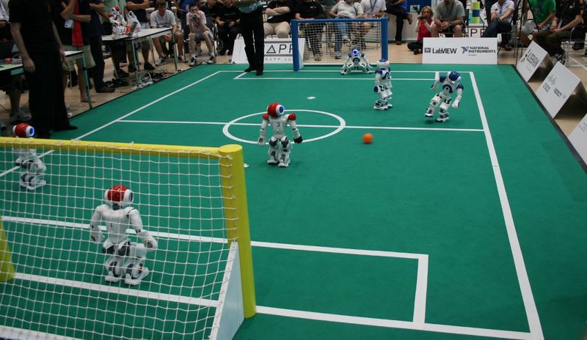
Since 2008, the humanoid robot Nao [1] that is manufac-
tured by the French company Aldebaran Robotics is the robot
used in the RoboCup Standard Platform League (cf. Fig. 1).
The Nao has 21 degrees of freedom (cf. Fig. 2 left). It is
equipped with a 500 MHz processor, two cameras, an inertial
measuring unit, sonar sensors in its chest, and force-sensitive
resistors under its feet.
Aldebaran Robotics provides a gait for the Nao [1] that
is based on keeping the center of mass of the robot above
the area supported by the feet. It is completely open-loop
resulting in a low robustness on surfaces such as the carpet Fig. 2. The joints of the Nao [1] (left). The robot coordinate system used
usually used in RoboCup. In addition, it only allows the user in this paper (right).
to choose between a pre-defined set of steps, i. e., it is not
omni-directional. This makes it hard to be used in RoboCup,
where precise and fast alignment behind the ball is a must.
RoboCup 2008, Kulk and Welch designed an open-loop walk
The maximum speed reached is approximately 10 cm/s. For
that keeps the stiffness of the joints as low as possible to both
conserve energy and to increase the stability of the walk [2].
The gait reached 14 cm/s. However, since it is still based on
the walking module provided by Aldebaran Robotics, it still
shares the major drawback of not being omni-directional. Two
groups worked on walks that keep the Zero Moment Point
(ZMP) [3] above the support area using preview controllers.
Both implement real omni-directional gaits. Czarnetzki et al.
[4] reached speeds up to 20 cm/s with their approach. In their
paper, this was only done in simulation. However, at RoboCup
2009 their robots reached similar speeds on the actual field,
but they seemed to be hard to control and there was a certain
lack in robustness, i. e., the robot fell down quite often. Strom
et. al [5] modeled the robot as an inverted pendulum in their
ZMP-based method. They reached speeds of around 10 cm/s.
Fig. 1. Naos on a soccer field at RoboCup 2009 in Graz. The main contributions of this paper are: we describe a
Proceedings of the 4th Workshop on Humanoid Soccer Robots
A workshop of the 2009 IEEE-RAS Intl. Conf. On Humanoid Robots (Humanoids 2009),
Paris(France), 2009, December 7-10
ISBN 978-88-95872-03-2
pp. 30-37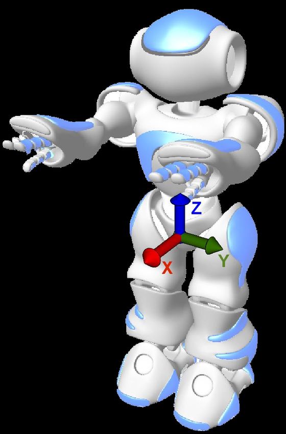
CoM-based gait for the Nao that is supported by strong                           Because of the nature of the kinematic chain, this transfor-
balancing methods resulting in a robust system, as proven in                     mation is inverted. Then the translational part of the transfor-
actual RoboCup games. We also describe an analytical solution                    mation is solely determined by the last three joints and hence
to the inverse kinematics of the Nao. To our knowledge, it is                    they can be computed directly.
the first one that was published so far, because in the work
described above, only iterative approaches are mentioned.                                      HipOrth2F oot = F oot2HipOrth−1                            (3)
Finally, we provide some practical insights in how the pose
                                                                                 The limbs of the leg and the knee form a triangle, in
of the robot’s torso can be estimated using the readings from
                                                                                 which an edge equals the length of the translation vector
the inertial board and we compare them to the pose estimation
                                                                                 of HipOrth2F oot (ltrans ). Because all three edges of this
provided by the inertia board itself.
                                                                                 triangle are known (the other two edges, the lengths of the
   The structure of this paper is as follows: first, we present
                                                                                 limbs, are fix properties of the Nao) the angles of the triangle
the analytical solution to the inverse kinematics of the Nao.
                                                                                 can be computed using the law of cosines (4). Knowing that
Then, our method for walking is presented, followed by
                                                                                 the angle enclosed by the limbs corresponds to the knee joint,
our approach to active balancing, which makes the gait a
                                                                                 that joint angle is computed by equation (5).
closed-loop solution. Since balancing is based on the pose
of the torso of the robot, the estimation pitch and roll of the                                     c2 = a2 + b2 − 2 · a · b · cos γ                      (4)
torso is described afterwards. The paper closes with a short
presentation of the results.                                                                             lupperLeg 2 + llowerLeg 2 − ltrans 2
                                                                                          γ = arccos                                                      (5)
                     II. I NVERSE K INEMATICS                                                                 2 · lupperLeg · llowerLeg
   Solving the inverse kinematics problem analytically for the                   Because γ represents an interior angle and the knee joint
Nao is not straightforward because of two special circum-                        is being streched in the zero-position, the resulting angle is
stances:                                                                         computed by
   • The axes of the hip yaw joints are rotated by 45 degrees                                           δknee = π − γ                       (6)
      (cf. Fig. 2).
   • These joints are also mechanically connected among both                     Additionally the angle opposite to the upper leg has to be
      legs, i. e., they are driven by a single servo motor.                      computed, because it corresponds to the foot pitch joint:
   The target of the feet is given as homogenous transforma-                                                                                         2
                                                                                                             llowerLeg 2 + ltrans 2 − lupperLeg
tion matrices, i. e., matrices containing the rotation and the                     δf ootP itch1 = arccos                                                 (7)
translation of the foot in the coordinate system of the torso.                                                      2 · llowerLeg · ltrans
To explain our solution we use the following convention:                         Now the foot pitch and roll joints combined with the triangle
A transformation matrix that transforms a point pA given                         form a kind of pan-tilt-unit. Their joints can be computed from
in coordinates of coordinate system A to the same point                          the translation vector using atan2.3
pB in coordinate system B is named A2B, so that pB =                                                                    p
A2B · pA . Hence the transformation matrix that describes the                                   δf ootP itch2 = atan2(x, y 2 + z 2 )          (8)
foot position relative to the torso is F oot2T orso that is given
as input. The coordinate frames used are depicted in Fig. 3.                                            δf ootRoll = atan2(y, z)                          (9)
   The position is given relative to the torso, i. e., more
                                                                                 where x, y, z are the components of the translation of
specifically relative to the center point between the intersection
                                                                                 F oot2HipOrth. As the foot pitch angle is composed by two
points of the axes of the hip joints. So first of all the position
                                                                                 parts it is computed as the sum of its parts.
relative to the hip is needed1 . This is a simple translation along
the y-axis2                                                                                    δf ootP itch = δf ootP itch1 + δf ootP itch2              (10)

                                    ldist
          F oot2Hip = T ransy                · F oot2T orso      (1)             After the last three joints of the kinematic chain (viewed
                                      2
                                                                                 from the torso) are determined, the remaining three joints
with ldist = distance between legs. Now the first problem                        that form the hip can be computed. The joint angles can
is solved by describing the position in a coordinate system                      be extracted from the rotation matrix of the hip that can be
rotated by 45 degrees, so that the axes of the hip joints can                    computed by multiplications of transformation matrices. For
be seen as orthogonal. This is achieved by a rotation around                     this purpose another coordinate frame T high is introduced that
the x-axis of the hip by 45 degrees or π4 radians.                               is located at the end of the upper leg, viewed from the foot.
                                         π                                       The rotation matrix for extracting the joint angles is contained
            F oot2HipOrth = Rotx ( ) · F oot2Hip                 (2)
                                         4                                       in HipOrth2T high that can be computed by
   1 The computation is described for one leg. Of course, it can be applied to
the other leg as well.                                                            HipOrth2T high = T high2F oot−1 · HipOrth2F oot (11)
   2 The    elementary     homogenous       transformation     matrices    for
rotation and translation are noted as Rot (angle) resp.                      3 atan2(y, x) is defined as in the C standard library, returning the angle
T rans (translation).                                                      between the x-axis and the point (x, y).
                                  Proceedings of the 4th Workshop on Humanoid Soccer Robots
                      A workshop of the 2009 IEEE-RAS Intl. Conf. On Humanoid Robots (Humanoids 2009),
                                               Paris(France), 2009, December 7-10
                                                     ISBN 978-88-95872-03-2
                                                            pp. 30-37
Fig. 3. Visualization of coordinate frames used in the inverse kinematic. From left to right: T orso, Hip, HipOrth, T high, F oot. The x-axis is shown
in red, the y-axis in green, and the z-axis in blue.
where T high2F oot can be computed by following the kine- position exactly. Given this fixed hip joint angle, there are
matic chain from foot to thigh. only five variable joints supposed to realize a 6DOF-pose,
thus it is impossible to reach the desired pose exactly. This
T high2F oot = Rotx (δf ootRoll ) · Roty (δf ootP itch )
is a typical optimization problem that we solved analytically
·T ransz (llowerLeg ) · Roty (δknee ) (12)
by introducing a virtual foot yaw joint at the end of the
·T ransz (lupperLeg )
kinematic chain. Now we have again six joints to realize a
To understand the computation of those joint angles, the 6DOF-pose which is, as described above, solvable analytically.
rotation matrix produced by the known order of hip joints This modified kinematic chain can be seen as reversed since
(yaw (z), roll (x), pitch (y)) is constructed (the matrix is noted the universal joint is now located at the foot and not at the torso
abbreviated, e. g. cx means cos δx ). anymore. Hence this modified inverse kinematic problem can
RotHip = Rotz (δz ) · Rotx (δx ) · Roty (δy ) be solved for each leg as described above. The only difference
cy cz − sx sy sz −cx sz cz sy + cy sx sz
is that the order of joints and the transformation of the foot
= cz sx sy + cy sz cx cz −cy cz sx + sy sz relative to the torso has to be inverted.
−cx sy sx cx cy The decision to introduce a foot yaw joint was mainly taken
(13) because an error in this (virtual) joint has a low impact on the
The angle δx can obviously be computed by arcsin r32 .4 The stability of the robot, whereas other joints (e. g. foot pitch or
extraction of δy and δz is more complicated, they must be roll) have a huge impact on stability.
computed using two entries of the matrix, which can be easily III. WALKING
seen by some transformation:
Walking means that the robot moves with desired speeds
−r12 cos δx · sin δz sin δz in forward, sideways, and rotational directions. To accomplish
= = = tan δz (14)
r22 cos δx · cos δz cos δz this, the two feet of the robot have to follow three-dimensional
Now δz and, using the same approach, δy can be computed trajectories that define the actual steps. In previous work [6],
by we determined the trajectories of the feet relative to the torso.
δz = δhipY aw = atan2(−r12 , r22 ) (15) However, in the approach presented here, the trajectories of the
feet are modeled relative to the center of mass (CoM). The foot
δy = δhipP itch = atan2(−r31 , r33 ) (16) positions relative to the CoM and the stance of the other body
At last the rotation by 45 degrees (cf. eq. 2) has to be parts are used for determining foot positions relative to the
compensated in joint space. torso that move the CoM to the desired point. Foot positions
π relative to the torso allow using inverse kinematics (cf. Sect. II)
δhipRoll = δx − (17) for the generation of joint angles.
4
Before the creation of walking motions starts, a stance (the
Now all joints are computed. This computation is done for stand) that will be used as basis for the foot joint angles during
both legs, assuming that there is an independent hip yaw joint the whole walking motion is required. This stance is called S
for each leg. The computation described above can lead to and it is created from foot positions relative to the torso using
different resulting values for the hip yaw joints of the left and inverse kinematics (cf. Sect. II). S is mirror-symmetrically to
the right leg. Given these two joint values, a single resulting x-z-plane of the robot’s coordinate system (cf. Fig. 2 right).
value is determined, the computation of which is dynamically For the temporal dimension, a phase ϕ that runs from 0 to
parameterized. This is necessary, because if the values differ, (excluding) 1 and repeats permanently is used. The phase can
only one leg can realize the desired target, and normally be separated into two half-phases, in each of which alternately
the support leg (cf. sect. III) is supposed to reach the target one leg is the support leg and the other one can be lifted up.
4 The first index denotes the row, the second index denotes the column of The size of each half-step is determined at the beginning of
the rotation matrix. each half-phase.
Proceedings of the 4th Workshop on Humanoid Soccer Robots
A workshop of the 2009 IEEE-RAS Intl. Conf. On Humanoid Robots (Humanoids 2009),
Paris(France), 2009, December 7-10
ISBN 978-88-95872-03-2
pp. 30-37a) p =0 b) p =0.5 c) p =0
a) phase
ϕ=0 b) phase
ϕ = 0.5 c) ϕphase
=0
sr
sl
sl sl
sr
sr sr
CoM
left foot
CoM
CoM right foot right foot
body
left foot right foot left foot
body body
Fig. 4. Illustration of the foot shifting within three half-phases from a top-down view. At first, the robot stands (a) and then it walks two half-steps to the
front (b, c). The support leg (left leg in (a)) changes in (b) and (c). Between (a) and (b), the step size sr is added to the right foot position. Between (b)
and (c), sr is subtracted from the right and left foot positions, so that the body moves forwards. Additionally, the new offset sr + sl is added to the left
foot position. The CoM visualized is the projection of the desired CoM position on the ground, that differs significantly from the respective projection of
the “center of body”. Therefore an additional offset has to be added to all translational components of both foot positions, to move the CoM to the desired
position.
The shifting of the feet is separated into the “shift”- and
“transfer”-phases. Both phases last a half-phase, run sequen- 1−cos(2π(2ϕ−x )/y )
l l
if 2ϕ ∈ ]xl . . . xl + yl [
tially, and are transposed for both feet. Within the “shift”- tlLif t = 2 (20)
0 otherwise
phase, the foot is lifted (“lift”-phase) and moved (“move”- 1−cos(2π(2ϕ−x )/y )
phase) to another place on the ground, so that the foot is
b l l
if 2ϕb ∈ ]xl . . . xl + yl [
trLif t = 2 (21)
completely shifted at the end of the phase. The foot-shifting is 0 otherwise
1−cos(π(2ϕ−x )/y )
subtracted from the foot position within the “transfer”-phase m m
if 2ϕ ∈
2
and also subtracted from the other foot position until that foot
]xm . . . xm + ym [
is shifted (cf. Fig. 4). This alone creates a motion that already tlM ove = 1 if 2ϕ ∈ (22)
looks like a walking motion. But the desired CoM movement
[x m + y m . . . 1[
is still missing.
0 otherwise
So the foot positions relative to the torso (plRel and prRel ) 1−cos(π(2ϕ−x
m )/ym )
b
2 if 2ϕb∈
are calculated as follows:
]xm . . . xm + ym [
trM ove = 1 if 2ϕb∈ (23)
[x + y . . . 1[
ol + slLif t · tlLif t
m m
0 otherwise
+sl · tlM ove
plRel = −sr · (1 − tlM ove ) · tl if ϕ < 0.5 (18)
1−cos(2πϕ)
if ϕ < 0.5
l + slLif t · tlLif t
o tl = 2 (24)
0 otherwise
+sl · (1 − tr ) otherwise
1−cos(2πϕ)
if ϕ ≥ 0.5
tr =
or + srLif t · trLif t 2 (25)
0 otherwise
+sr · trM ove
prRel = −sl · (1 − trM ove ) · tr if ϕ ≥ 0.5 (19) The CoM movement has to be performed along the y-axis
o r + srLif t · trLif t
as well as in walking direction. The CoM is already moving
in walking direction by foot shifting, but this CoM movement
+sr · (1 − tl ) otherwise
does not allow walking with a speed that meets our needs.
ol and or are the foot origin positions. slLif t and srLif t Also, a CoM movement along the z-axis is useful. First of all,
are the total offsets used for lifting either the left or the the foot positions relative to the CoM are determined by using
right leg. sl and sr are the current step sizes. tlLif t and the foot positions relative to the CoM of stance S and adding
trLif t are parameterized trajectories that are used for the foot the value of a trajectory to the y-coordinate of these positions.
lifting. They are parameterized with the beginning (xl ) and the Since the calculated foot positions are relative to the CoM, the
duration (yl ) (cf. Fig. 5) of the “lift”-phase. tlM ove and trM ove rotation of the body that can be added with another trajectory
are used for adding the step sizes. They are parameterized with has to be considered for the calculation of the foot positions.
the beginning (xm ) and the duration (ym ) of the “move”- The CoM movement in x-direction is calculated with the help
phase (cf. Fig. 6). tl and tr are shifted cosine shapes used of the step sizes of the currently performed half-steps.
for subtracting the step sizes (cf. Fig. 7). The trajectories are If any kind of body and foot rotations and CoM-lifting along
defined as follows (ϕ b = ϕ − 1): the z-axis are ignored, the desired foot positions relative to the
Proceedings of the 4th Workshop on Humanoid Soccer Robots
A workshop of the 2009 IEEE-RAS Intl. Conf. On Humanoid Robots (Humanoids 2009),
Paris(France), 2009, December 7-10
ISBN 978-88-95872-03-2
pp. 30-371 tcom tcom
tlLift s(ps(ϕ)
phase)
1 r(pr(ϕ)
phase)
l(pl(ϕ)
phase)
0.8 0.5
0.6
0
0.4
-0.5
0.2 xl xl+yl
-1
0
0 0.2 0.4 0.6 0.8 1
0 0.2 0.4 0.6 0.8 1 ϕ
pphase
2ϕ
2•pphase
Fig. 8. The trajectory tcom that is used for the CoM movement along the
Fig. 5. The trajectory tlLif t that is used for foot lifting. trLif t is similar y-axis. It is a composition of s(ϕ), r(ϕ) and l(ϕ).
to tlLif t except that it is shifted one half-phase to the right.
CoM (plCom and prCom ) can be calculated as follows:
tlMove
1
−cS + ss · tcom + ol
0.8
plCom = − sl ·tlin −s2r ·(1−tlin ) if ϕ < 0.5 (26)
prCom − prRel + plRel otherwise
0.6
−cS + ss · tcom + or
prCom = − sr ·tlin −s2l ·(1−tlin ) if ϕ ≥ 0.5 (27)
plCom − plRel + prRel otherwise
0.4
cS is the offset to the CoM relative to the torso of the
0.2 xm xm+ym
stance S. ss is the vector that describes the amplitude of the
CoM movement along the y-axis. tcom is the parameterized
0 trajectory of the CoM movement. Therefore, a sine (s(p)),
0 0.2 0.4 0.6 0.8 1 square root of sine (r(p)) and a linear (l(p)) component are
2ϕ
2•pphase
merged according to the ratios xc (for s(p)), yc (for r(p)) and
zc (for l(p)) (cf. Fig. 8). tcom is defined as:
Fig. 6. The trajectory tlM ove that is used for adding step sizes. trM ove is
similar to tlM ove except that it is shifted one half-phase to the right.
xc · s(ϕ) + yc · r(ϕ) + zc · l(ϕ)
tcom = (28)
xc + yc + zc
tl
1 s(p) = sin(2πp) (29)
p
r(p) = |sin(2πp)| · sgn(sin(2πp)) (30)
0.8
4p if p < 0.25
l(p) = 2 − 4p if p ≥ 0.25 ∧ p < 0.75 (31)
4p − 4 if p ≥ 0.75
0.6
tlin is a simple linear trajectory used for moving the CoM
0.4 into the walking direction.
2ϕ if ϕ < 0.5
0.2 tlin = (32)
2ϕ − 1 if ϕ ≥ 0.5
0
Based on the desired foot positions relative to the CoM,
0 0.2 0.4 0.6 0.8 1 another offset is calculated and added to the foot positions
2ϕ
2•pphase
relative to the torso (plRel and prRel ) to achieve the desired
foot positions relative to the CoM with coordinates relative to
Fig. 7. The trajectory tl that is used for subtracting step sizes. tr is similar
to tl except that it is shifted one half-phase to the right. the torso. For the calculation of the additional offset, the fact
that the desired CoM position does not change significantly
Proceedings of the 4th Workshop on Humanoid Soccer Robots
A workshop of the 2009 IEEE-RAS Intl. Conf. On Humanoid Robots (Humanoids 2009),
Paris(France), 2009, December 7-10
ISBN 978-88-95872-03-2
pp. 30-37between two cycles is exploited, because the offset that was C. Phase Balancing
determined in the previous frame is used first. So, given the Balancing by modifying the walking phase is another possi-
current leg, arm, and head stance and the offset of the previous bility. Therefore, the measured x-angle, the expected x-angle
frame, foot positions relative to the CoM are determined. The and the current walking phase position are used to determine
difference between these foot positions and the desired foot a measured phase position. The measured position allows
positions is added to the old offset to get the new one. The calculating the error between the measured and actual phase
resulting foot positions relative to the CoM are not precise, position. This error can be used for adding an offset to the
but the error is negligible. current phase position. When the phase position changes in
The additional offset (enew ) can be calculated using the old this manner, the buffered desired foot positions and body
offset (eold ) as follows: rotations have to be adjusted, because the modified phase
plRel −plCom +prRel −prCom position affects the desired foot positions and body rotations
enew = 2 (33) of the past.
−ceold ,plRel ,prRel
D. Step-Size Balancing
ceold ,plRel ,prRel is the CoM offset relative to the torso given
the old offset, the new foot stance, and the stance of the other Step-size balancing is the last supported kind of balancing.
limbs. It works by increasing or decreasing the step size during the
Finally, plRel − enew and prRel − enew are the positions execution of half-steps according to the foot position error
used for creating the joint angles, because: that was already used for CoM Balancing. Applied step-size
balancing has the disadvantage that the predicted odometry
offset becomes imprecise. Therefore, it can be deactivated for
plRel − cenew ,plRel ,prRel − enew ≈ plCom (34) critical situations such as when positioning for kicking the
prRel − cenew ,plRel ,prRel − enew ≈ prCom (35) ball.
IV. BALANCING V. T ORSO P OSE E STIMATION
To react on unexpected events and for stabilizing the walk Estimating the pose of the torso consists of three different
in general, balancing is required. Therefore, several balancing tasks. First, discontinuities in the inertial sensor readings are
methods are supported. Three of them are simple p-controllers. excluded. Second, the calibration offsets for the two gyro-
Only the step-size balancing also has an integral component. scopes (x and y, cf. Fig. 2 right for the robot coordinate system
The error that is used as input for the controllers is solely used in this paper) are maintained. Third, the actual torso pose
determined from the actual pose of the robot torso, i. e., the is estimated using an Unscented Kalman filter (UKF) [7].
pitch and roll angles of the torso relative to the ground, and Excluding discontinuities in the sensor readings is neces-
the expected pose. The delay between the measured and the sary, because some sensor measurements provided by the Nao
desired CoM positions is taken into account by buffering cannot be explained by the usual sensor noise. This malfunc-
and restoring the desired foot positions and torso poses. The tion occurs sporadically and affects most measurements from
different kinds of balancing are: the inertial measuring unit within a single frame (cf. Fig. 9).
The corrupted frames are detected by comparing the difference
A. CoM Balancing of each value and its predecessor to a predefined threshold. If
The CoM balancer works by adding an offset to the a corrupted frame is found that way, all sensor measurements
desired foot positions (plCom and prCom ). Therefore, the from the inertial measuring unit are ignored. Corrupted ac-
error between the measured and desired foot positions has celerometer values are replaced with their predecessors and
to be determined, so that the controller can add an offset to corrupted gyroscope measurements are simply not used.
these positions according to the determined error. The error is Gyroscopes have a bias drift, i. e., the output when the
calculated by taking the difference between the desired foot angular velocity is zero drifts over time due to factors such as
positions and the same positions rotated according to rotation temperature that cannot be observed. The temperature changes
error. slowly as long as the robot runs, so that it is necessary to re-
determine the bias continuously. Therefore, it is hypothesized
B. Rotation Balancing that the torso of the robot and thereby the inertial measurement
Besides CoM Balancing, it is also possible to balance with unit has the same pose at the beginning and the end of a
the body and/or foot rotation. Therefore, angles depending on walking phase (i. e. two steps). Therefore, the average gyro
the rotation error can be added to the target foot rotations measurement over a whole walking phase should be zero.
or can be used for calculating the target foot positions and This should also apply if the robot is standing. So either,
rotations. This affects the CoM position, so that the offset the average measurements over a whole walking phase are
computation that is used for moving the foot positions relative determined, or the average over 1 sec for a standing robot.
to the CoM might compensate the balancing impact. So this These averages are filtered through one-dimensional Kalman
kind of balancing probably makes only sense when it is filters and used as biases of the gyroscopes. The collection of
combined with CoM Balancing. gyroscope measurements is limited to situations in which the
Proceedings of the 4th Workshop on Humanoid Soccer Robots
A workshop of the 2009 IEEE-RAS Intl. Conf. On Humanoid Robots (Humanoids 2009),
Paris(France), 2009, December 7-10
ISBN 978-88-95872-03-2
pp. 30-37UKF, but also to get a “filtered” version of the gyroscope
measurements from the change in orientation, including a
calculated z-gyroscope value that is actually missing on the
Nao.
VI. R ESULTS
The gait described here was used at RoboCup 2009 by the
team B-Human [8] in the Standard Platform League – the
world champion and winner of the technical challenge. The
maximum speeds reached in soccer competitions were 15 cm/s
forwards, 10 cm/s backwards, 9 cm/s sideways, and 35◦ /s
rotational speed. An interesting effect is that the theoretical
maximum forward speed resulting from the foot trajectories
generate is only 12 cm/s. The additional 3 cm/s seem to
Fig. 9. A typical corrupted inertia sensor reading between the frames 110 result from balancing by changing the step size. Therefore it
and 100. The corrupted data was detected and replaced with its predecessor.
seems that the robot is walking faster because it continuously
prevents itself from falling down to the front.
At RoboCup 2009, our walk was the most robust one
for the Nao, and it still was among the fastest walks. Its
precision made us the team that was able to most quickly
align behind the ball for kicking. As a result we scored more
goals than all the other 23 teams in the Standard Platform
League together. There is a video on the B-Human homepage
(http://www.b-human.de) showing some scenes from
the games in which the gait can be seen. The software used
by B-Human at RoboCup 2009 can also be downloaded from
that website, including the implementation of the algorithms
described in this paper.
VII. C ONCLUSION AND F UTURE W ORK
In this paper we presented a CoM-based closed-loop gait
for the Nao. Four different balancing methods make the gait
very robust, as has been proven during the RoboCup 2009
competitions. We also described an analytical solution to the
inverse kinematics of the Nao that is used for our gait. Finally,
we described the estimation of the pose of the robot’s torso,
Fig. 10. The difference between the estimated pitch angle angleY and the which is the reference for the balancing methods.
pitch angle rawAngleY provided by the inertia board of the Nao. Higher speeds can be achieved with this approach, but so
far not in a way that would allow walking omni-directionally
for more than 10 minutes in a row (a half-time) without falling
robot is either standing or walking slowly and has contact to down. Hence, we will replace the CoM-based core of our gait
the ground (determined through the force-sensitive resistors in with a ZMP-based preview controller in the future, carefully
Nao’s feet). keeping the balancing methods in place that are the main
The UKF estimates the pose of the robot torso (cf. Fig. 10) reasons for the robustness of the current walk. In addition,
that is represented as three-dimensional rotation matrix. The we will work on automatically optimizing the parameters of
change of the rotation of the feet relative to the torso in each our gait, using Particle Swarm Optimization (PSO) [9] as we
frame is used as process update. The sensor update is derived have already done for a Kondo robot [10]. Actually, a few
from the calibrated gyroscope values. Another sensor update is parameters of the gait presented in this paper were already
added from a simple absolute measurement realized under the optimized using this method.
assumption that the longer leg of the robot rests evenly on the
ground as long as the robot stands almost upright. In cases in ACKNOWLEDGEMENTS
which this assumption is apparently incorrect, the acceleration
sensor is used instead. The authors would like to thank all B-Human team members
It is not only possible to get the orientation from the for providing the software base for this work.
Proceedings of the 4th Workshop on Humanoid Soccer Robots
A workshop of the 2009 IEEE-RAS Intl. Conf. On Humanoid Robots (Humanoids 2009),
Paris(France), 2009, December 7-10
ISBN 978-88-95872-03-2
pp. 30-37R EFERENCES
[1] D. Gouaillier, V. Hugel, P. Blazevic, C. Kilner, J. Monceaux, P. Lafour-
cade, B. Marnier, J. Serre, and B. Maisonnier, “The NAO hu-
manoid: a combination of performance and affordability,” CoRR, vol.
abs/0807.3223, 2008.
[2] J. A. Kulk and J. S. Welsh, “A low power walk for the NAO robot,”
in Proceedings of the 2008 Australasian Conference on Robotics &
Automation (ACRA-2008), J. Kim and R. Mahony, Eds., 2008.
[3] M. Vukobratovic and B. Borovac, “Zero-moment point – thirty five years
of its life,” International Journal of Humanoid Robotics, vol. 1, no. 1,
pp. 157–173, 2004.
[4] S. Czarnetzki, S. Kerner, and O. Urbann, “Observer-based dynamic
walking control for biped robots,” Robotics and Autonomous Systems,
vol. 57, no. 8, pp. 839–845, 2009.
[5] J. Strom, G. Slavov, and E. Chown, “Omnidirectional walking using
ZMP and preview control for the nao humanoid robot,” in RoboCup
2009: Robot Soccer World Cup XIII, ser. Lecture Notes in Artificial
Intelligence, J. Baltes, M. G. Lagoudakis, T. Naruse, and S. Shiry, Eds.
Springer, to appear in 2010.
[6] T. Röfer, T. Laue, A. Burchardt, E. Damrose, K. Gillmann,
C. Graf, T. J. de Haas, A. Härtl, A. Rieskamp, A. Schreck,
and J.-H. Worch, “B-Human team report and code release 2008,”
2008, 72 pages. [Online]. Available: http://www.b-human.de/media/
coderelease08/bhuman08 coderelease.pdf
[7] S. J. Julier, J. K. Uhlmann, and H. F. Durrant-Whyte, “A new approach
for filtering nonlinear systems,” in American Control Conference, 1995.
Proceedings of the, vol. 3, 1995, pp. 1628–1632. [Online]. Available:
http://ieeexplore.ieee.org/xpls/abs all.jsp?arnumber=529783
[8] T. Röfer, T. Laue, O. Bösche, I. Sieverdingbeck, T. Wiedemeyer,
and J.-H. Worch, “B-Human team description for robocup 2009,” in
RoboCup 2009: Robot Soccer World Cup XII Preproceedings, J. Baltes,
M. Lagoudakis, T. Naruse, and S. Shiry, Eds. RoboCup Federation,
2009.
[9] R. C. Eberhart and J. Kennedy, “A new optimizer using particles swarm
theory,” in Sixth International Symposium on Micro Machine and Human
Science, 1995, pp. 39–43.
[10] C. Niehaus, T. Röfer, and T. Laue, “Gait optimization on a humanoid
robot using particle swarm optimization,” in Proceedings of the Second
Workshop on Humanoid Soccer Robots in conjunction with the 2007
IEEE-RAS International Conference on Humanoid Robots, C. Zhou,
E. Pagello, E. Menegatti, and S. Behnke, Eds., 2007.
Proceedings of the 4th Workshop on Humanoid Soccer Robots
A workshop of the 2009 IEEE-RAS Intl. Conf. On Humanoid Robots (Humanoids 2009),
Paris(France), 2009, December 7-10
ISBN 978-88-95872-03-2
pp. 30-37You can also read