Across the Time Dimension in Search of Exotic Particles - Max Goncharov for CDF Collaboration
←
→
Page content transcription
If your browser does not render page correctly, please read the page content below
Across the Time Dimension in Search of
            Exotic Particles
     Max Goncharov for CDF Collaboration
In This Talk ...
    Massive Long Lived Particles
     general things we do not understand, evidence for
     something out there, some theories and signatures

    CDF Detector
     Time-of-Flight (TOF), Track Timing (COT), EMTiming

    Charged Massive Particles (a.k.a. CHAMPs)
     results from CDF with 1 fb-1

    Neutral Massive Particles (a.k.a. delayed photons)
     results from CDF with 0.6 fb-1

    Where we would like to go
     tools we developed, things we learned. new ideas
2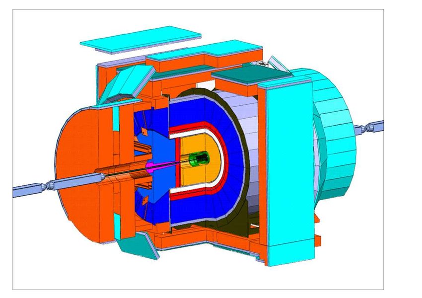
Why Search Beyond SM?
       Standard Model is great, but some questions linger
                 Only 3 generations?
                 Why so different masses?
                 No antimatter?
                 Dark Matter?!

    mt=175 GeV

         Colliding Galaxies: while normal matter (red) slows down
         the dark matter (blue) keeps going as if nothing happened
3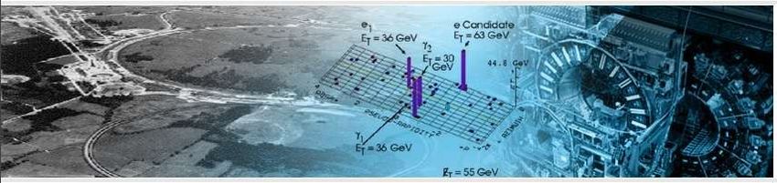
Massive and LongLived
X
~ 1/F1/2 F
X mG =
3 M pl
(NLSP) ~
G (LSP)
Wide variety of models:
➢ m(G) ~ 100200 GeV
➢ G is good dark matter candidate
➢ small m=m X => large lifetime
−m G
SUSY (GMSB) model:
➢ neutralino – NLSP, m(G) ~ 10 KeV
➢ neutralino lifetime is unconstrained
4
Stable Massive Particles
Standard Model extensions predict new massive particles
Most searches assume particles decay promptly
Long-lived particles would evade these searches
• Charged Massive Particles (CHAMPs)
• Neutral Stable Massive Particles decaying to photons
In perfect life all Standard Model backgrounds are zero
Often need to develop new tools
all backgrounds are estimated from data
blind analysis (learn how to estimate backgrounds, then look at
the data in the signal region)
model-independent results (but also set limits)
5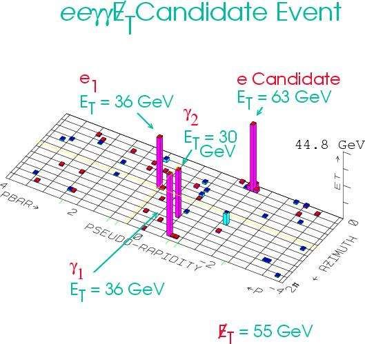
Stable Massive Exotic Particles
Can decay:
inside the detector
outside the detector
They can be:
charged or neutral
be in events with low PT
long lifetime
What
large mass
low speed
cold relic
6
Possible Signatures
CHAMP – charged massive particle
highly ionizing/late track
decaying inside the detector:
delayed photons
signatures should be spectacular
7
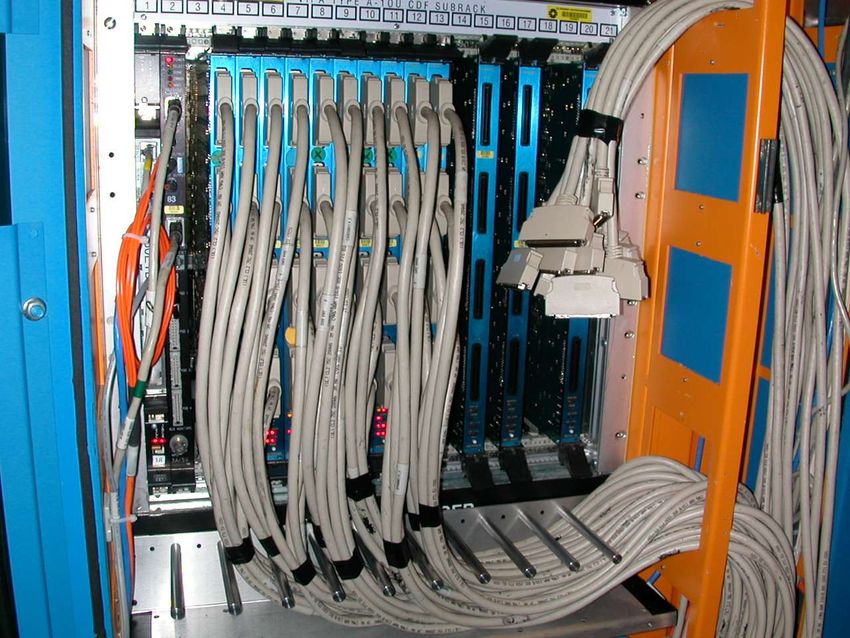
CDF Detector
                                                   Electromagnetic
                                                   Calorimeter (EM)

                                                             CDF

                                                          TOF

                               Hadronic
                                            Tracking    Muon
                              Calorimeter   Chamber    Detector

      CHAMPs – tracking, calorimeters, TOF, muon
      Delayed Photons – tracking, EM calorimeter

8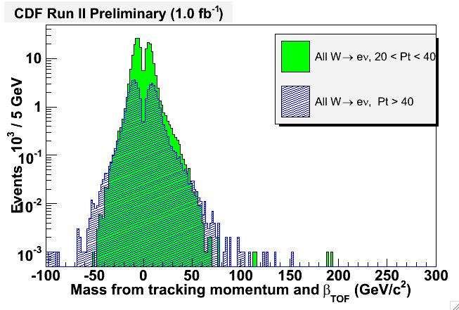
Time of Flight Detector
Muon Detectors TOF – scintillators wrapped
around tracking chamber (COT) at
a 1.45 m
Timing Resolution – 100 ps
Use Time-of Flight (TOF) detector
to measure β for charged particles
To calculate β, need:
• candidate TOF arrival time
• independent interaction t0
• path length
≡v /c
9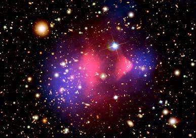
Time Measurement with COT
● Drift chamber is a timing device
● Each Track produces up to 96 hits
● Each hit has timing information
● Up to 96 time measurements on a track
Potentially lots of timing information
Large statistics can compensate for low single-hit
precision (for a track, resolution ~ 200 ps)
Measure arrival times at wire planes and cell
boundaries
• Can measure track velocity with or without event t0
Gaussian tails!
10New Tool – EMTiming System
Adding timing to EM Calorimeter would help
• Photon handle: provide a vitally important handle that
confirms or denies that all the photons in unusual
events are from the primary collision.
• Met handle: for events with large EM energy, full
calorimeter coverage reduces the cosmic ray and
beam halo background sources and improves the
sensitivity for high-PT physics such as SUSY, LED,
Anomalous Couplings etc.
• Search for long-live particles
11New Tool EMTiming System
~2000 Phototubes
• Large system to add to existing
detector (Run IIb upgrade)
• Put a TDC onto about 2000
phototubes at CDF ( || < 2 )
• TDC has 1 ns buckets
• for central detector use passive
inductive pick-off to split PMT anode
signal
published in NIM
http://hepr8.physics.tamu.edu/hep/emtiming/
12Luminosity
400 pb1 600 pb1 ~100% Efficient above thresholds
(CEM-5, PEM-2.5 GeV)
EMTiming system installed System resolution is ~0.6 ns
Very uniform
Negligible Noise
Finished full installation October
2004. Started taking data in
November (1.4 fb-1 and counting)
Commissioned in 1 week
All high PT events have timing
information
13CHAMP Signature
Champs give a unique signature in the detector
CHAMPs are heavy
Slow ≡v /c1
Hard to stop
CHAMPs are slow
Large dE/dx (mostly through ionization) dE / dX ~1/ 2
Long time-of-flight
Look for high transverse momentum (PT) penetrating
objects (looks like muon) that are slow (long time-of-
flight)
14CHAMP Signal Isolation
Use track momentum and velocity
measurements to calculate mass
● correlated for signal, uncorrelated for background
Signal events will have large momentum
● signal region PT > 40 GeV/c
● control region 20 GeV/c < PT < 40 GeV/c
● use control region to predict background shape
120 GeV Stop
180 GeV Stop
15Analysis Strategy
It is the mass of the muons we are after
m= p 1/ β −1
● use beta shape in the the control region as a shape
2
● convolute it with the momentum
Show this works for electrons from Ws
● sanity check take electrons with 20 < P < 40 GeV
T
● beta shape + momentum histogram = background prediction
● agrees with data
Show we can predict electrons with PT > 40 GeV
Muons:
● split control region in 2: 20 < P < 30 and 30 < P < 40
T T
● show that can predict 2 from 1
● get beta shape for 20 < P < 40
T
● make prediction for PT > 40 GeV, compare with data in the signal
region
16Backgrounds
Cosmic rays
● Time of cosmic ray tracks uncorrelated with interaction time,
could appear to be CHAMPs
● Remove by looking for backward-going track opposite
candidate (identified by timing as well)
Instrumental effects: t Flight =t TOF −t Event
Mismeasured event t0
require TOF and tracking t0 to agree (0.5 ns)
Incorrect TOF for CHAMP candidate
require good COT χ2 when using TOF β
Mismeasured momentum
can get hight mass for a 6 TeV track with β = 1
17 require β significantly different from 1 (β < 0.9)Electrons Sample
● Nice place to understand mass
calculation
● Use electron momentum
β > 1 unphysical
p assign negative mass to “tachyons”
m= p 1/ β −12
β mass
18Check With Electrons
Assume p and β are independent
● Calculate mass bin-by-bin from p
and β histograms
● weight by bin contents
● gives mass shape prediction
Works!
● p and β are largely independent in
the control sample
Predictions generated from
control-region β and signal-
region p
Assume β matches in both
regions
19Muon Control Region
Require central muons ( || < 0.6 )
Verify background shape prediction
● use 20-30 GeV to predict 30-40 GeV region
20CHAMPs – Signal Region
No CHAMP candidates above 120 GeV/c2. Signal-
region events consistent with background prediction
21Model Independent Limits
For model independence, find cross section limit for
CHAMPs fiducial to Central Muon Detectors with
0.4< β < 0.9 and Pt > 40 GeV
– strongly interacting (stable stop)
● efficiency 4.6 ±0.5%
● 95% confidence limit: σ < 41 fb
– weakly interacting (sleptons, charginos)
● efficiency 20.0±0.6%
● 95% confidence limit: σ < 9.4 fb
Model-dependent factors are
– β and momentum distributions
– geometric acceptance
22New Stable Stop Limits
L = 53/pb
Exclude Stable Stop with mass
below 250 GeV/c2 (95% C.L.)
Excluded by ALEPH
23When We Find CHAMPs
If a mass peak is observed in the CHAMP search,
we have many additional handles to prove these
are slow particles:
– Calorimeter timing
– Muon timing
– dE/dx
24Break
Moving into neutral heavy longlived particles
25Why Photons?
Run I
• In addition to γγ+ Energy
Imbalance this event has
two high energy electron
candidates
• Very unusual
• Total Background:
(1 ± 1) x 10-6 Events
Would be nice to have timing for the photons to prove they
are from collision
26Delayed Photons + Jet + MET
Monte Carlo
Signal
Look for non-prompt 's that take
longer to reach calorimeter.
If the 0 has a significant lifetime, we
Photon Time of Arrival
can separate the signal from the
backgrounds. Standard Model
27Analysis Strategy
Sample gamma + Jet + MET
look for photons that are late
Want to understand time shapes from various backgrounds
Noncollision backgrounds
● general shape from notrack events
● separate beam halo from cosmics
Standard Model Background
● event T0 dominates the resolution – have to subtract
● background splits in two
● guessed the primary vertex correctly
● guessed the primary vertex incorrectly
We use data in various control regions to normalize shapes and obtain
background prediction in the signal region
28Delayed Photons
Standard Model
Beam Halo Signal Monte Carlo Four Background Sources
Noncollision “looklike photons”
Cosmics • Cosmics
• Beam Halo
Collision photons from Standard
Model
• Right vertex
• Wrong vertex
Signal (Blinded) Region [2 10] ns
29Backgrounds
Beam Halo Muon – in sync with beam
Cosmic Ray
If two interactions – how do we
know where photons come from?
We don't!
?
P P
we trigger on photons
Tracks – PT and time are measured by
the tracking chamber => can reconstruct
event origin in time
30NonCollision Backgrounds
● There are lots of tracks in typical collision.
● Non-collision means there are no tracks.
● Cosmics are accidents - flat in time
● What about beam halo?
● Most would choose |T| < 6 ns
● We use shapes predictions
gate opens .... closes
31Cosmics vs Beam Halo
Tracks PT < 1 GeV
N
Ha
dro
nic Proton Direction
To we r s Cosmics
we N EM To
rs Beam Halo
32Beam Halo Time Shape 33
Timing Resolutions
This is how one normally measures
W> e true system resolution:
Z> ee
RMS = 0.6 ns
WHEN interaction happens RMS1.3 ns
It has to be subtracted from the photon arrival time
Need to reconstruct vertices in space and time
34Collision Time Reconstruction
For tracks we reconstruct Z position along the beamline and time as
measured by the tracking drift chamber (COT):
plot all tracks on ZTime plane
Separating those two is what do clustering
we are after.
Track Time (ns)
RMS = 1.28 ns
Track Z (cm)
35Standard Model Photons
Assigning the right vertex is a tricky business as L gets high
We can measure how often mistake is made
Electrons
Standard Model (SM) photon
candidates
• Right vertex
• Wrong vertex
When wrong vertex picked:
= 2 e 2 vertex =
1.6 1.3 ≃2.05 ns
2 2
With electrons we simulate what happens with photons
by excluding electron track from vertex reconstruction
36Putting It All Together
Normalize shapes to data outside the blind region
Control Regions:
+ MET + jets Cosmics : 30 80 ns
Beam Halo: 20 6 ns
Collisions : 6 1.2 ns
Optimize for best sensitivity:
Photon ET>30 GeV
Jet ET>35 GeV
MET>40 GeV
signal (blinded) region
37Delayed Photons
+ MET + jets
Predicted: 1.3 0.7 events
Observed: 2 events
Would be +6 event
for GMSB point:
m() = 100 GeV
() = 5 ns
We know shapes
normalize to events in control regions
count events in signal region (210) ns
38Delayed Photons?
95% C.L.
Did not find anything, but have
the highest sensitivity
39Analysis with More Data
more data is available
40What is Next?
CHAMPs 0.4 Delayed Photons
Late Tracks
Track Timing
Calorimeter Timing
Non-Collision Rejection
Space-Time vertex Exclusive +MET
(KK states ...)
Champs Backup Slides 42
Outlook
                   Understand Collisions,
                                                   Popular exotic signature:
                       Track timing,
                                                   2Photons + MET
                  Cosmics and Beam Effects

                  CHAMPs         Delayed Photons

      Escaping Susy     Delayed Jets   Displaced Vertices

43
Model Independent Limits 44
Supersymmetry:
stable stop squark (We use this as our reference model)
R. Barbieri, L.J. Hall and Y. Nomura PRD 63, 105007 (2001)
NLSP stau in gauge-mediated SUSY breaking
J.L. Feng, T. Moroi, Phys.Rev. D58 (1998) 035001
Light strange-beauty squarks
• K. Cheung and W-S. Hou, Phys.Rev. D70 (2004) 035009
Light strange-beauty squarks
• Matthew Strassler, HEP-ph/0607160
Universal Extra Dimensions (UXDs)
Kaluza-Klein modes of SM particles
T. Appelquist, H-C. Cheng, B.A. Dobrescu, PRD 64 (2001) 035002
Long-lived 4th generation quarks
• P.H. Frampton, P.Q. Hung, M. Sher, Phys. Rep. 330 (2000) 263-348.
45Reasons to live
Particles can be long-lived if they have:
• weak coupling constants
• limited phase space
• a conserved quantity
• “hidden valley” (potential barrier)
46Beam Longitudinal Width
p and p-bar bunches have different width =>
collision time is correlated with the collision location
Z
Average z position of the interaction is given by
Z = exp((zct)2/2(p))*exp((zct)2/2(pbar))
(p) = 55 cm
(pbar) = 65 cm
47Stable Stop
Look at Stable Stop (reference model)
R. Barbieri, L.J. Hall and Y. Nomura PRD 63, 105007 (2001)
Pair produced
– Get kinematic and geometric acceptance
• Pt > 40 GeV; 0.9 > β > 0.4; TOF Fiducial
– Must be charged:
• in tracking chamber for identification
• in muon detectors for trigger
Statistical + Systematic Errors
Statistical + Systematic Errors
48Speed of Light with Beam Halo
Beamhalo Primary Collision
BeamHalo path
Measure speed of beamhalo to be 2*108 m/s
49Which Model to Pick? 50
You can also read