Adversarial Regularizers in Inverse Problems
←
→
Page content transcription
If your browser does not render page correctly, please read the page content below
Adversarial Regularizers in Inverse Problems

                                                 Sebastian Lunz                  Ozan Öktem                      Carola-Bibiane Schönlieb
                                                    DAMTP                  Department of Mathematics                     DAMTP
                                             University of Cambridge    KTH - Royal Institute of Technology       University of Cambridge
                                              Cambridge CB3 0WA                100 44 Stockholm                    Cambridge CB3 0WA
                                             lunz@math.cam.ac.uk                 ozan@kth.se                        cbs31@cam.ac.uk
arXiv:1805.11572v2 [cs.CV] 11 Jan 2019

                                                                                       Abstract
                                                   Inverse Problems in medical imaging and computer vision are traditionally solved
                                                   using purely model-based methods. Among those variational regularization models
                                                   are one of the most popular approaches. We propose a new framework for applying
                                                   data-driven approaches to inverse problems, using a neural network as a regular-
                                                   ization functional. The network learns to discriminate between the distribution of
                                                   ground truth images and the distribution of unregularized reconstructions. Once
                                                   trained, the network is applied to the inverse problem by solving the corresponding
                                                   variational problem. Unlike other data-based approaches for inverse problems,
                                                   the algorithm can be applied even if only unsupervised training data is available.
                                                   Experiments demonstrate the potential of the framework for denoising on the BSDS
                                                   dataset and for computed tomography reconstruction on the LIDC dataset.

                                         1     Introduction
                                         Inverse problems naturally occur in many applications in computer vision and medical imaging. A
                                         successful classical approach relies on the concept of variational regularization [11, 24]. It combines
                                         knowledge about how data is generated in the forward operator with a regularization functional that
                                         encodes prior knowledge about the image to be reconstructed.
                                         The success of neural networks in many computer vision tasks has motivated attempts at using deep
                                         learning to achieve better performance in solving inverse problems [15, 2, 25]. A major difficulty
                                         is the efficient usage of knowledge about the forward operator and noise model in such data driven
                                         approaches, avoiding the necessity to relearn the physical model structure.
                                         The framework considered here aims to solve this by using neural networks as part of variational
                                         regularization, replacing the typically hand-crafted regularization functional with a neural network.
                                         As classical learning methods for regularization functionals do not scale to the high dimensional
                                         parameter spaces needed for neural networks, we propose a new training algorithm for regularization
                                         functionals. It is based on the ideas in Wasserstein generative adversarial models [5], training the
                                         network as a critic to tell apart ground truth images from unregularized reconstructions.
                                         Our contributions are as follows:

                                                1. We introduce the idea of learning a regularization functional given by a neural network,
                                                   combining the advantages of the variational formulation for inverse problems with data-
                                                   driven approaches.
                                                2. We propose a training algorithm for regularization functionals which scales to high dimen-
                                                   sional parameter spaces.
                                                3. We show desirable theoretical properties of the regularization functionals obtained this way.
                                                4. We demonstrate the performance of the algorithm for denoising and computed tomography.

                                         32nd Conference on Neural Information Processing Systems (NeurIPS 2018), Montréal, Canada.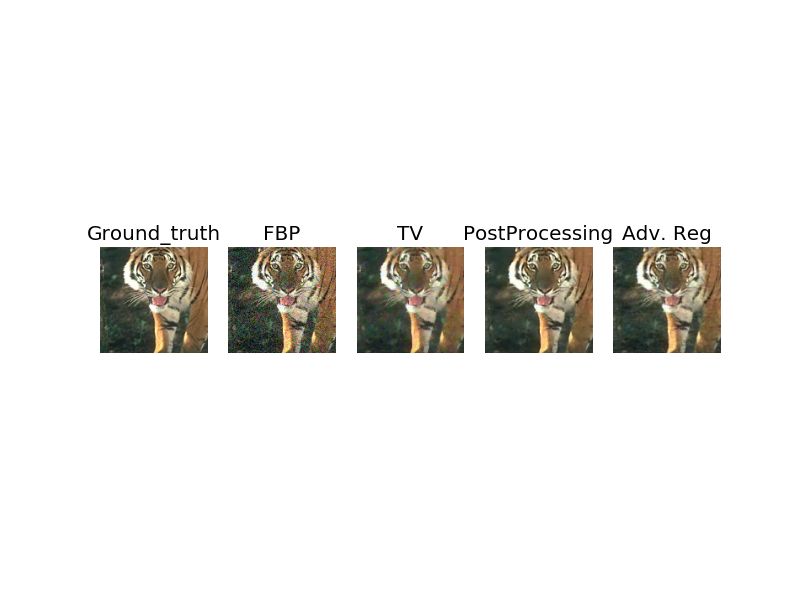
2     Background
2.1   Inverse Problems in Imaging

Let X and Y be reflexive Banach spaces. In a generic inverse problem in imaging, the image x ∈ X
is recovered from measurement y ∈ Y , where
                                             y = Ax + e.                                            (1)
A : X → Y denotes the linear forward operator and e ∈ Y is a random noise term. Typical
tasks in computer vision that can be phrased as inverse problems include denoising, where A is the
identity operator, or inpainting, where A is given by a projection operator onto the complement of
the inpainting domain. In medical imaging, common forward operators are the Fourier transform in
magnetic resonance imaging (MRI) and the ray transform in computed tomography (CT).

2.2   Deep Learning in Inverse Problems

One approach to solve (1) using deep learning is to directly learn the mapping y → x using a neural
network. While this has been observed to work well for denoising and inpainting [28], the approach
can become infeasible in inverse problems involving forward operator with a more complicated
structure [4] and when only very limited training data is available. This is typically the case in
applications in medical imaging.
Other approaches have been developed to tackle inverse problems with complex forward operators. In
[15] an algorithm has been suggested that first applies a pseudo-inverse to the operator A, leading to
a noisy reconstruction. This result is then denoised using deep learning techniques. Other approaches
[1, 14, 25] propose applying a neural network iteratively. Learning proximal operators for solving
inverse problems is a further direction of research [2, 19].

2.3   Variational regularization

Variational regularization is a well-established model-based method for solving inverse problems.
Given a single measurement y, the image x is recovered by solving
                                    argminx kAx − yk22 + λf (x),                                    (2)
where the data term kAx −    yk22
                                ensures consistency of the reconstruction x with the measurement y
and the regularization functional f : X → R allows us to insert prior knowledge onto the solution
x. The functional f is usually hand-crafted, with typical choices including total variation (TV) [23]
which leads to piecewise constant images and total generalized variation (TGV) [16], generating
piecewise linear images.

3     Learning a regularization functional
In this paper, we design a regularization functional based on training data. We fix a-priori a class
of admissible regularization functionals F and then learn the choice {f }f ∈F from data. Existing
approaches to learning a regularization functionals are based on the idea that f should be chosen such
that a solution to the variational problem
                                    argminx kAx − yk22 + λf (x),                                    (3)
best approximates the true solution. Given training samples (xj , yj ), identifying f using this method
requires one to solve the bilevel optimization problem [17, 9]
                       X
          argminf ∈F       kx˜j − xj k2 , subject to x̃j ∈ argminx kAx − yj k22 + f (x).             (4)
                        j

But this is computationally feasible only for small sets of admissible functions F. In particular, it
does not scale to sets F parametrized by some high dimensional space Θ.
We hence apply a novel technique for learning the regularization functional f ∈ F that scales to high
dimensional parameter spaces. It is based on the idea of learning to discriminate between noisy and
ground truth images.

                                                   2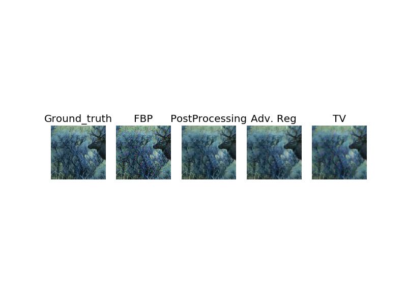
In particular, we consider approaches where the regularization functional is given by a neural network
ΨΘ with network parameters Θ. In this setting, the class F is given by the functions that can be
parametrized by the network architecture of Ψ for some choice of parameters Θ. Once Θ is fixed, the
inverse problem (1) is solved by
                                   argminx kAx − yk22 + λΨΘ (x).                                     (5)

3.1   Regularization functionals as critics

Denote by xi ∈ X independent samples from the distribution of ground truth images Pr and by
yi ∈ Y independent samples from the distribution of measurements PY . Note that we only use
samples from both marginals of the joint distribution PX×Y of images and measurement, i.e. we are
in the setting of unsupervised learning.
The distribution PY on measurement space can be mapped to a distribution on image space by
applying a -potentially regularized- pseudo-inverse A†δ . In [15] it has been shown that such an inverse
can in fact be computed efficiently for a large class of forward operators. This in particular includes
Fourier and ray transforms occurring in MRI and CT. Let
                                            Pn = (A†δ )# PY
be the distribution obtained this way. Here, # denotes the push-forward of measures, i.e.
A†δ Y ∼ (A†δ )# PY for Y ∼ PY . Samples drawn from Pn will be corrupted with noise that both
depends on the noise model e as well as on the operator A.
A good regularization functional ΨΘ is able to tell apart the distributions Pr and Pn - taking high
values on typical samples of Pn and low values on typical samples of Pr [7]. It is thus clear that
                                 EX∼Pr [ΨΘ (X)] − EX∼Pn [ΨΘ (X)]
being small is desirable. With this in mind, we choose the loss functional for learning the regularizer
to be
                                                             h                        i
                                                                                    2
               EX∼Pr [ΨΘ (X)] − EX∼Pn [ΨΘ (X)] + λ · E (k∇x ΨΘ (X)k − 1)+ .                         (6)

The last term in the loss functional serves to enforce the trained network ΨΘ to be Lipschitz continuous
with constant one [13]. The expected value in this term is taken over all lines connecting samples in
Pn and Pr .
Training a neural network as a critic was first proposed in the context of generative modeling in
[12]. The particular choice of loss functional has been introduced in [5] to train a critic that captures
the Wasserstein distance between the distributions Pr and Pn . A minimizer to (6) approximates a
maximizer f to the Kantorovich formulation of optimal transport [26].
                    Wass(Pr , Pn ) =     sup      EX∼Pn [f (X)] − EX∼Pr [f (X)] .                    (7)
                                       f ∈1−Lip

Relaxing the hard Lipschitz constraint in (7) into a penalty term as in (6) was proposed in [13].
Tracking the gradients of ΨΘ for our experiments demonstrates that this way the Lipschitz constraint
can in fact be enforced up to a small error.

Algorithm 1 Learning a regularization functional
Require: Gradient penalty coefficient µ, batch size m, Adam hyperparameters α, inverse A+
                                                                                        δ
  while Θ has not converged do
    for i ∈ 1, ..., m do
      Sample ground truth image xr ∼ Pr , measurement y ∼ PY and random number  ∼ U [0, 1]
      x n ← A+  δ y
      xi = xr + (1 − )xn
                                                         2
      Li ← ΨΘ (xr ) − ΨΘ (xn ) + µ (k∇xi ΨΘ (xi )k − 1)+
    end for            Pm
    Θ ← Adam(∇Θ i=1 Li , α)
  end while

                                                    3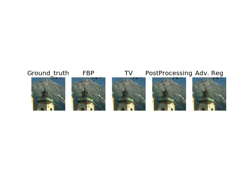
Algorithm 2 Applying a learned regularization functional with gradient descent
Require: Learned regularization functional ΨΘ , measurements y, regularization weight λ, step size
   , operator A, inverse A+δ , Stopping criterion S
   x ← A+   δ y
   while S not satisfied
                       do
      x ← x − ∇x kAx − yk22 + λΨΘ (x)
   end while
   return x
In the proposed algorithm, gradient descent is used to solve (5). As the neural network is in general
non-convex, convergence to a global optimum cannot be guaranteed. However, stable convergence to
a critical point has been observed in practice. More sophisticated algorithms like momentum methods
or a forward-backward splitting of data term and regularization functional can be applied [10].

3.2    Distributional Analysis

Here we analyze the impact of the learned regularization functional on the induced image distribution.
More precisely, given a noisy image x drawn from Pn , consider the image obtained by performing a
step of gradient descent of size η over the regularization functional ΨΘ
                                     gη (x) := x − η · ∇x ΨΘ (x).                                   (8)
This yields a distribution Pη := (gη )# Pn of noisy images that have undergone one step of gradient
descent. We show that this distribution is closer in Wasserstein distance to the distribution of ground
truth images Pr than the noisy image distribution Pn . The regularization functional hence introduces
the highly desirable incentive to align the distribution of minimizers of the regularization problem (5)
with the distribution of ground truth images.
Henceforth, assume the network ΨΘ has been trained to perfection, i.e. that it is a 1-Lipschitz function
which achieves the supremum in (7). Furthermore, assume ΨΘ is almost everywhere differentiable
with respect to the measure Pn .
Theorem 1. Assume that η 7→ Wass(Pr , Pη ) admits a left and a right derivative at η = 0, and that
they are equal. Then,
                        d
                           Wass(Pr , Pη )|η=0 = −EX∼Pn k∇x ΨΘ (X)k2 .

                       dη

Proof. The proof follows [5, Theorem 3]. By an envelope theorem [20, Theorem 1], the existence of
the derivative at η = 0 implies
                       d                       d
                          Wass(Pr , Pη )|η=0 =    EX∼Pn [ΨΘ (gη (X))]|η=0 .                         (9)
                       dη                      dη
On the other hand, for a.e. x ∈ X one can bound
      d
         ΨΘ (gη (x)) = |h∇x ΨΘ (gη (x)), ∇x ΨΘ (x)i| ≤ k∇x ΨΘ (gη (x)k · k∇x ΨΘ (x)k ≤ 1,          (10)
      dη
for any η ∈ R. Hence, in particular the difference quotient is bounded
                                    1
                                      [ΨΘ (gη (x)) − ΨΘ (x)] ≤ 1                                   (11)
                                    η
for any x and η. By dominated convergence, this allows us to conclude
                    d                                 d
                       EX∼Pn [ΨΘ (gη (X))]|η=0 = EX∼Pn [ΨΘ (gη (X))]|η=0 .                         (12)
                    dη                                dη
Finally,
                              d
                                 [ΨΘ (gη (X))]|η=0 = −k∇x ΨΘ (X)k2 .                               (13)
                              dη

                                                   4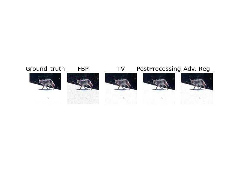
Remark 1. Under the weak assumptions in [13, Corollary 1], we have k∇x ΨΘ (x)k = 1, for Pn a.e.
x ∈ X. This allows to compute the rate of decay of Wasserstein distance explicitly to
                                   d
                                      [ΨΘ (gη (X))]|η=0 = −1                              (14)
                                  dη
Note that the above calculations also show that the particular choice of loss functional is optimal
in terms of decay rates of the Wasserstein distance, introducing the strongest incentive to align
the distribution of reconstructions with the ground truth distribution amongst all regularization
functionals. To make this more precise, consider any other regularization functional f : X → R with
norm-bounded gradients, i.e. k∇f (x)k ≤ 1.
Corollary 1. Denote by g̃η (x) = x − η · ∇f (x) the flow associated to f . Set P̃η := (g̃η )# (Pn ).
Then
                     d                               d
                        Wass(Pr , P̃η )|η=0 ≥ −1 =      Wass(Pr , Pη )|η=0                     (15)
                    dη                              dη

Proof. An analogous computation as above shows
  d
     Wass(Pr , P̃η )|η=0 = −EX∼Pn [h∇x ΨΘ (x), ∇x f (x)i] ≥ −1 = −EX∼Pn k∇x ΨΘ (X)k2 .

  dη

3.3   Analysis under data manifold assumption

Here we discuss which form of regularization functional is desirable under the data manifold
assumption and show that the loss function (6) in fact gives rise to a regularization functional
of this particular form.
Assumption 1 (Weak Data Manifold Assumption). Assume the measure Pr is supported on the
weakly compact set M, i.e. Pr (Mc ) = 0
This assumption captures the intuition that real data lies in a curved lower-dimensional subspace of
X.
If we consider the regularization functional as encoding prior knowledge about the image distribution,
it follows that we would like the regularizer to penalize images which are away from M. An extreme
way of doing this would be to set the regularization functional as the characteristic function of M.
However, this choice of functional comes with two major disadvantages: First, solving (5) with
methods based on gradient descent becomes impossible when using such a regularization functional.
Second, the functional effectively leads to a projection onto the data manifold, possibly causing
artifacts due to imperfect knowledge of M [8].
An alternative to consider is the distance function to the data manifold d(x, M), since such a choice
provides meaningful gradients everywhere. This is implicitly done in [21]. In Theorem 2, we show
that our chosen loss function in fact does give rise to a regularization functional ΨΘ taking the
desirable form of the l2 distance function to M.
Denote by
                            PM : D → M,        x → argminy∈M kx − yk                              (16)
the data manifold projection, where D denotes the set of points for which such a projection exists.
We assume Pn (D) = 1. This can be guaranteed under weak assumptions on M and Pn .
Assumption 2. Assume the measures Pr and Pn satisfy
                                         (PM )# (Pn ) = Pr                                        (17)
                                                  −1
i.e. for every measurable set A ⊂ X, we have Pn (PM  (A)) = Pr (A)
We hence assume that the distortions of the true data present in the distribution of pseudo-inverses Pn
are well-behaved enough to recover the distribution of true images from noisy ones by projecting back
onto the manifold. Note that this is a much weaker than assuming that any given single image can be
recovered by projecting its pseudo-inverse back onto the data manifold. Heuristically, Assumption 2
corresponds to a low-noise assumption.

                                                  5
Theorem 2. Under Assumptions 1 and 2, a maximizer to the functional
sup EX∼Pn f (X) − EX∼Pr f (X) (18)
f ∈1−Lip
is given by the distance function to the data manifold
dM (x) := min kx − yk (19)
y∈M
Proof. First show that dM is Lipschitz continuous with Lipschitz constant 1. Let x1 , x2 ∈ X be
arbitrary and denote by ỹ a minimizer to miny∈M kx2 − yk2 . Indeed,
dM (x1 ) − dM (x2 ) = min kx1 − yk − min kx2 − yk = min kx1 − yk − kx2 − ỹk
y∈M y∈M y∈M
≤ kx1 − ỹk − kx2 − ỹk ≤ kx1 − x2 k,
where we used the triangle inequality in the last step. This proves Lipschitz continuity by exchanging
the roles of x1 and x2 .
Now, we prove that dM obtains the supremum in 18. Let h be any 1-Lipschitz function. By
assumption 2, one can rewrite
EX∼Pn [h(X)] − EX∼Pr [h(X)] = EX∼Pn [h(X) − h(PM (X))] . (20)
As h is 1 Lipschitz, this can be bounded via
EX∼Pn [h(X) − h(PM (X))] ≤ EX∼Pn [kX − PM (X)k] . (21)
The distance between x and PM (x) is by definition given by dM (x). This allows to conclude via
EX∼Pn [kX − PM (X)k] = EX∼Pn [dM (X)] = EX∼Pn [dM (X) − dM (PM (X))]
= EX∼Pn [dM (X)] − EX∼Pr [dM (X)] .
Remark 2 (Non-uniqueness). The functional (18) does not necessarily have a unique maximizer.
For example, f can be changed to an arbitrary 1-Lipschitz function outside the convex hull of
supp(Pr ) ∩ supp(Pn ).
4 Stability
Following the well-developed stability theory for classical variational problems [11], we derive a
stability estimate for the adversarial regularizer algorithm. The key difference to existing theory is
that we do not assume the regularization functional f is bounded from below. Instead, this is replaced
by a 1 Lipschitz assumption on f .
Theorem 3 (Weak Stability in Data Term). We make Assumption 3. Let yn be a sequence in Y with
yn → y in the norm topology and denote by xn a sequence of minimizers of the functional
argminx∈X kAx − yn k2 + λf (x)
Then xn has a weakly convergent subsequence and the limit x is a minimizer of kAx − yk2 + λf (x).
The assumptions and the proof are contained in Appendix A.
5 Computational Results
5.1 Parameter estimation
Applying the algorithm to new data requires choosing a regularization parameter λ. Making the
assumption that the ground truth images are critical points of the variational problem (5), λ can
be estimated efficiently from the noise level, using the fact that the regularization functional has
gradients of unit norm. This leads to the formula
λ = 2 Ee∼pn kA∗ ek2 ,
where A∗ denotes the adjoint and pn the noise distribution. In all experiments, the regularization
parameter has been chosen according to this formula without further tuning.
6Table 1: Denoising results on BSDS dataset
Method PSNR (dB) SSIM
Noisy Image 20.3 .534
M ODEL - BASED
Total Variation [23] 26.3 .836
S UPERVISED
Denoising N.N. [28] 28.8 .908
U NSUPERVISED
Adversarial Regularizer (ours) 28.2 .892
(a) Ground Truth (b) Noisy Image (c) TV (d) Denoising N.N. (e) Adversarial Reg.
Figure 1: Denoising Results on BSDS
5.2 Denoising
As a toy problem, we compare the performance of total variation denoising [23], a supervised
denoising neural network approach [28] based on the UNet [22] architecture and our proposed
algorithm on images of size 128 × 128 cut out of images taken from the BSDS500 dataset [3]. The
images have been corrupted with Gaussian white noise. We report the average peak signal-to-noise
ratio (PSNR) and the structural similarity index (SSIM) [27] in Table 1.
The results in Figure 1 show that the adversarial regularizer algorithm is able to outperform classical
variational methods in all quality measures. It achieves results of comparable visual quality than
supervised data-driven algorithms, without relying on supervised training data.
5.3 Computed Tomography
Computer Tomography reconstruction is an application in which the variational approach is very
widely used in practice. Here, it serves as a prototype inverse problem with non-trivial forward
operator. We compare the performance of total variation [18, 23], post-processing [15], Regular-
ization by Denoising (RED) [21] and our proposed regularizers on the LIDC/IDRI database [6] of
lung scans. The denoising algorithm underlying RED has been chosen to be the denoising neural
network previously trained for post-processing. Measurements have been simulated by taking the ray
transform, corrupted with Gaussian white noise. With 30 different angles taken for the ray transform,
the forward operator is undersampled. The code is available online 1 .
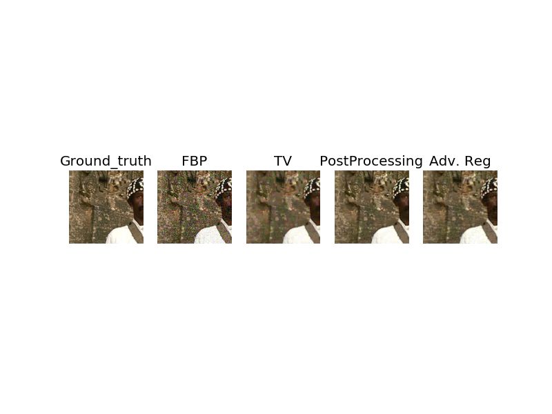
The results on different noise levels can be found in Table 2 and Figure 2, with further examples in
Appendix C. Note in Table 2 that Post-Processing has been trained with PSNR as target loss function.
Again, total variation is outperformed by a large margin in all categories. Our reconstructions are of
the same or superior visual quality than the ones obtained with supervised machine learning methods,
despite having used unsupervised data only.
6 Conclusion
We have proposed an algorithm for solving inverse problems, using a neural network as regulariza-
tion functional. We have introduced a novel training algorithm for regularization functionals and
showed that the resulting regularizers have desirable theoretical properties. Unlike other data-based
1
https://github.com/lunz-s/DeepAdverserialRegulariser
7Table 2: CT reconstruction on LIDC dataset
(a) High noise (b) Low noise
Method PSNR (dB) SSIM Method PSNR (dB) SSIM
M ODEL - BASED M ODEL - BASED
Filtered Backprojection 14.9 .227 Filtered Backprojection 23.3 .604
Total Variation [18] 27.7 .890 Total Variation [18] 30.0 .924
S UPERVISED S UPERVISED
Post-Processing [15] 31.2 .936 Post-Processing [15] 33.6 .955
RED [21] 29.9 .904 RED [21] 32.8 .947
U NSUPERVISED U NSUPERVISED
Adversarial Reg. (ours) 30.5 .927 Adversarial Reg. (ours) 32.5 .946
(a) Ground Truth (b) FBP (c) TV (d) Post-Processing (e) Adversarial Reg.
Figure 2: Reconstruction from simulated CT measurements on the LIDC dataset
approaches in inverse problems, the proposed algorithm can be trained even if only unsupervised
training data is available. This allows to apply the algorithm to situations where -due to a lack of
appropriate training data- machine learning methods have not been used yet.
The variational framework enables us to effectively insert knowledge about the forward operator and
the noise model into the reconstruction, allowing the algorithm to be trained on little training data. It
also comes with the advantages of a well-developed stability theory and the possibility of adapting
the algorithms to different noise levels by changing the regularization parameter λ, without having to
retrain the model from scratch.
The computational results demonstrate the potential of the algorithm, producing reconstructions of
the same or even superior visual quality as the ones obtained with supervised approaches on the LIDC
dataset, despite the fact that only unsupervised data has been used for training. Classical methods
like total variation are outperformed by a large margin.
Our approach is particularly well-suited for applications in medical imaging, where usually very few
training samples are available and ground truth images to a particular measurement are hard to obtain,
making supervised algorithms impossible train.
7 Extensions
The algorithm admits some extensions and modifications.
• Local Regularizers. The regularizer is restricted to act on small patches of pixels only,
giving the value of the regularization functional by averaging over all patches. This allows
to harvest many training samples from a single image, making the algorithm trainable on
even less training data. Local Adversarial Regularizers can be implemented by choosing a
neural network architecture consisting of convolutional layers followed by a global average
pooling.
• Recursive Training. When applying the regularization functional, the variational problem
has to be solved. In this process, the regularization functional is confronted with partially
reconstructed images, which are neither ground truth images nor exhibit the typical noise
distribution the regularization functional has been trained on. By adding these images to the
8samples the regularization functional is trained on, the neural network is enabled to learn
from its own outputs. First implementations show that this can lead to an additional boost in
performance, but that the choice of which images to add is very delicate.
8 Acknowledgments
We thank Sam Power, Robert Tovey, Matthew Thorpe, Jonas Adler, Erich Kobler, Jo Schlemper,
Christoph Kehle and Moritz Scham for helpful discussions and advice.
The authors acknowledge the National Cancer Institute and the Foundation for the National Institutes
of Health, and their critical role in the creation of the free publicly available LIDC/IDRI Database
used in this study. The work by Sebastian Lunz was supported by the EPSRC grant EP/L016516/1
for the University of Cambridge Centre for Doctoral Training, the Cambridge Centre for Analysis
and by the Cantab Capital Institute for the Mathematics of Information. The work by Ozan Öktem
was supported by the Swedish Foundation for Strategic Research grant AM13-0049. Carola-Bibiane
Schönlieb acknowledges support from the Leverhulme Trust project on ‘Breaking the non-convexity
barrier’, EPSRC grant Nr. EP/M00483X/1, the EPSRC Centre Nr. EP/N014588/1, the RISE projects
CHiPS and NoMADS, the Cantab Capital Institute for the Mathematics of Information and the Alan
Turing Institute.
References
[1] Jonas Adler and Ozan Öktem. Solving ill-posed inverse problems using iterative deep neural
networks. Inverse Problems, 33(12), 2017.
[2] Jonas Adler and Ozan Öktem. Learned primal-dual reconstruction. IEEE Transactions on
Medical Imaging, 37(6):1322–1332, 2018.
[3] Pablo Arbelaez, Michael Maire, Charless Fowlkes, and Jitendra Malik. Contour detection and
hierarchical image segmentation. IEEE Trans. Pattern Anal. Mach. Intell., 33(5).
[4] Maria Argyrou, Dimitris Maintas, Charalampos Tsoumpas, and Efstathios Stiliaris. Tomo-
graphic image reconstruction based on artificial neural network (ANN) techniques. In Nuclear
Science Symposium and Medical Imaging Conference (NSS/MIC). IEEE, 2012.
[5] Martín Arjovsky, Soumith Chintala, and Léon Bottou. Wasserstein generative adversarial
networks. International Conference on Machine Learning, ICML, 2017.
[6] Samuel Armato, Geoffrey McLennan, Luc Bidaut, Michael McNitt-Gray, Charles Meyer,
Anthony Reeves, Binsheng Zhao, Denise Aberle, Claudia Henschke, Eric Hoffman, et al.
The lung image database consortium (LIDC) and image database resource initiative (IDRI): a
completed reference database of lung nodules on ct scans. Medical physics, 38(2), 2011.
[7] Martin Benning, Guy Gilboa, Joana Sarah Grah, and Carola-Bibiane Schönlieb. Learning filter
functions in regularisers by minimising quotients. In International Conference on Scale Space
and Variational Methods in Computer Vision. Springer, 2017.
[8] Ashish Bora, Ajil Jalal, Eric Price, and Alexandros Dimakis. Compressed sensing using
generative models. arXiv preprint arXiv:1703.03208, 2017.
[9] Luca Calatroni, Chung Cao, Juan Carlos De Los Reyes, Carola-Bibiane Schönlieb, and Tuomo
Valkonen. Bilevel approaches for learning of variational imaging models. RADON book series,
8, 2012.
[10] Antonin Chambolle and Thomas Pock. An introduction to continuous optimization for imaging.
Acta Numerica, 25, 2016.
[11] Heinz Werner Engl, Martin Hanke, and Andreas Neubauer. Regularization of inverse problems,
volume 375. Springer Science & Business Media, 1996.
[12] Ian Goodfellow, Jean Pouget-Abadie, Mehdi Mirza, Bing Xu, David Warde-Farley, Sherjil
Ozair, Aaron Courville, and Yoshua Bengio. Generative adversarial nets. In Advances in neural
information processing systems (NIPS), 2014.
[13] Ishaan Gulrajani, Faruk Ahmed, Martin Arjovsky, Vincent Dumoulin, and Aaron Courville.
Improved training of wasserstein GANs. Advances in Neural Information Processing Systems
(NIPS), 2017.
9[14] Kerstin Hammernik, Teresa Klatzer, Erich Kobler, Michael Recht, Daniel Sodickson, Thomas
Pock, and Florian Knoll. Learning a variational network for reconstruction of accelerated MRI
data. Magnetic resonance in medicine, 79(6), 2018.
[15] Kyong Hwan Jin, Michael McCann, Emmanuel Froustey, and Michael Unser. Deep convolu-
tional neural network for inverse problems in imaging. IEEE Transactions on Image Processing,
26(9), 2017.
[16] Florian Knoll, Kristian Bredies, Thomas Pock, and Rudolf Stollberger. Second order total
generalized variation (TGV) for MRI. Magnetic Resonance in Medicine, 65(2), 2011.
[17] Karl Kunisch and Thomas Pock. A bilevel optimization approach for parameter learning
iniational models. SIAM Journal on Imaging Sciences, 6(2), 2013.
[18] Rowan Leary, Zineb Saghi, Paul Midgley, and Daniel Holland. Compressed sensing electron
tomography. Ultramicroscopy, 131, 2013.
[19] Tim Meinhardt, Michael Moeller, Caner Hazirbas, and Daniel Cremers. Learning proximal
operators: Using denoising networks for regularizing inverse imaging problems. In International
Conference on Computer Vision (ICCV), 2017.
[20] Paul Milgrom and Ilya Segal. Envelope theorems for arbitrary choice sets. Econometrica, 70(2),
2002.
[21] Yaniv Romano, Michael Elad, and Peyman Milanfar. The little engine that could: Regularization
by denoising (RED). SIAM Journal on Imaging Sciences, 10(4), 2017.
[22] Olaf Ronneberger, Philipp Fischer, and Thomas Brox. U-net: Convolutional networks for
biomedical image segmentation. In International Conference on Medical Image Computing
and Computer-Assisted Intervention. Springer, 2015.
[23] Leonid I Rudin, Stanley Osher, and Emad Fatemi. Nonlinear total variation based noise removal
algorithms. Physica D: nonlinear phenomena, 60(1-4), 1992.
[24] Otmar Scherzer, Markus Grasmair, Harald Grossauer, Markus Haltmeier, and Frank Lenzen.
Variational methods in imaging. Springer, 2009.
[25] Jo Schlemper, Jose Caballero, Joseph V Hajnal, Anthony Price, and Daniel Rueckert. A
deep cascade of convolutional neural networks for mr image reconstruction. In International
Conference on Information Processing in Medical Imaging. Springer, 2017.
[26] Cédric Villani. Optimal transport: old and new, volume 338. Springer Science & Business
Media, 2008.
[27] Zhou Wang, Alan Bovik, Hamid Sheikh, and Eero Simoncelli. Image quality assessment: from
error visibility to structural similarity. IEEE transactions on image processing, 13(4), 2004.
[28] Junyuan Xie, Linli Xu, and Enhong Chen. Image denoising and inpainting with deep neural
networks. In Advances in Neural Information Processing Systems (NIPS), 2012.
10Appendix
A Stability Theory
Assumption 3. All of the following three conditions hold true.
• f is lower semi-continuous with respect to the weak topology on X and 1 Lipschitz with
respect to the metric induced by the norm.
• A is continuous or equivalently weak-to-weak continuous
• One of the following two conditions hold true
kAxk
– 0 < α := inf x kxk
– kf (x)k → ∞ as kxk → ∞
These assumptions are standard in the classical stability theory for inverse problems [11], with the
difference that we assume f to be 1 Lipschitz instead of being bounded from below.
Next we show that in the particular setting S = dM where dM is the distance function to the manifold
M, the weak continuity assumption on is always satisfied.
Lemma 1. The map dM is weakly lower semi-continuous.
Proof. Let xn be a sequence in X with xn → x weakly. Pick any subsequence of xn , for convenience
still denoted by xn . Denote by yn elements in M such that
dM (xn ) = min kxn − yk = kxn − yn k.
y∈M
As all yn ∈ M, we can extract a weakly convergent subsequence, denoted by ynj , such that ynj → y
weakly for some y ∈ M. By lower semi-continuity of the norm, estimate
lim inf dM (xnj ) = lim inf kxnj − ynj k ≥ kx − yk ≥ min kx − yk = dM (x) (22)
j→∞ j→∞ y∈M
Lemma 2 (Coercivity). Let y ∈ Y . Then under assumptions 3,
kAx − yk2 + λf (x) → ∞
as kxk → ∞, uniformly in all y ∈ Y with kyk ≤ 1.
kAxk
Proof. Assume first 0 < α := inf x kxk . WLOG assume kxk ≥ α−1 . Then
kAx − yk2 + λf (x) ≥ (αkxk − 1)2 + λ(f (x) − f (0) + f (0))
≥ (αkxk − 1)2 − λkxk + f (0) → ∞
as kxk → ∞, uniformly in y with kyk ≤ 1. The last inequality uses the assumption that f is 1
Lipschitz.
In the case kS(x)k → ∞ as kxk → ∞ the statement follows immediately.
Theorem 4 (Existence of Minimizer). Under assumptions 3, there exists a minimizer of
kAx − yk2 + λf (x).
Proof. Let xn be a sequence in X such that
kAxn − yk2 + λf (xn ) → min kAx − yk2 + λf (x)
x∈X
as n → ∞. Then by Lemma 2, xn is bounded in norm allowing to extract a weakly convergent
subsequence xn → x. As the norm is weakly lower-semi continuous and so is f by assumption, we
obtain
min kAx − yk2 + λf (x) = lim inf kAxn − yk2 + λf (xn ) ≥ kAx − yk2 + λf (x)
x∈X n→∞
thus proving that x is indeed a minimizer.
11Theorem 5 (Weak Stability in Data Term). Assume 3. Let yn be a sequence in Y with yn → y in the
norm topology and denote by xn a sequence of minimizers of the functional
argminx∈X kAx − yn k2 + λf (x)
Then xn has a weakly convergent subsequence and the limit x is a minimizer of kAx − yk2 + λf (x).
Proof. By Lemma 2, the sequence kxn k is bounded and hence contains a weakly convergent subse-
quence xn → x. Note that the map L(y) = minx kAx − yk2 + λf (x) is continuous with respect to
the norm topology. On the other hand, as A is by assumption weak to weak continuous and both the
norm and f are weakly lower semi-continuous, the overall loss L(x, y) = kAx − yk2 + λf (x) is
weakly lower semi-continuous, so
lim inf L(xn , yn ) ≥ L(x, y).
n→∞
Together we obtain
L(y) = lim L(yk ) = lim L(xk , yk ) ≥ L(x, y), (23)
k→∞ k→∞
proving that the limit point x is indeed a minimizer of kAx − yk2 + λf (x).
B Implementation details
We used a simple 8 layer convolutional neural network with a total of four strided convolution layers
with stride 2, leaky ReLU (α = 0.1) activations and two final dense layer for all experiments with
the adversarial regularizer algorithm. The network was optimized with RMSProp. We solved the
variational problem using gradient descent with fixed step size. The regularization parameter was
chosen according to the heuristic given in paper.
The comparison experiments with Post-Processing and the Denoising Neural Network used a UNet
style architecture, with four down-sampling (strided convolution, stride 2) and four up-sampling
(transposed convolution) convolutional layers with skip-connections after every down-sampling step
to the corresponding up-sampled layer of the same image resolution. Again, leaky ReLU activations
were used. The network was optimized using Adam. As training loss we used the `2 distance to the
ground truth, with no further regularization terms on the network parameters.
In the experiments with total variation, the regularization parameter was chosen using line search,
picking the parameter that leads to the best PSNR value. The minimization problem was solved using
primal-dual hybrid gradient descent (PDHG) [10].
12C Further Computational Results
Figure 3: Further denoising results on BSDS dataset.
From left to right: Ground truth, Noisy Image, TV, Denoising Neural Network, Adversarial Reg.
13Figure 4: Further CT reconstructions on LIDC dataset, high noise.
From left to right: Ground truth, FBP, TV, Post-Processing, Adversarial Reg.
(a) Ground Truth (b) Total Variation (c) Adversarial Regularizer
Figure 5: Adversarial Regularizers cause fewer artifacts around-small angle intersections of different
domains than TV. Results obtained for CT Reconstruction on synthetic ellipse data.
14Figure 6: Further CT reconstructions on LIDC dataset, low noise.
From left to right: Ground truth, FBP, TV, Post-Processing, Adversarial Reg.
Below the Sinogram used for reconstruction of the images.
15You can also read


