Adverse Weather Scenarios for Future Electricity Systems

Adverse Weather
Scenarios for Future
Electricity Systems:
Characterising short-duration
ramping events (including
addendum)
Author(s): Megan Pearce, Dr Laura Dawkins and Isabel Rushby
Reviewed by: Dr Emily Wallace

Prepared for: National Infrastructure Commission
Revision Date: February 2022

If printing double-sided you will need this blank page. If printing single sided, please delete
this page

 Page 2 of 79
© Crown copyright 2022, Met Office

Revision History

VERSION DESCRIPTION AUTHOR REVIEWER APPROVED
 FINAL (OCT 2021) Revisions finalised and Megan Emily Emily Wallace
 published Pearce, Wallace
 Additional sensitivity studies Laura
FINAL_WITHADDENDUM (DEC added Dawkins Emily Wallace
2021) Emily
 Wallace
 Megan
 Pearce,
 Laura
 Dawkins,
 Isabel
 Rushby

FINAL_WITHADDENDUM_REVISED Revisions made to remove Megan Emily Emily
 (FEB 2022) spurious midnight ramps Pearce, Wallace Wallace
 Laura
 Dawkins,
 Isabel
 Rushby

 Page 3 of 79
© Crown copyright 2022, Met Office

Disclaimer

 • This document is published by the Met Office on behalf of the Met Office on behalf of
 the Secretary of State for Business, Energy and Industrial Strategy, HM Government,
 UK. Its content is covered by © Crown Copyright 2022.
 • This document is published specifically for the readership and use of National
 Infrastructure Commission and may not be used or relied upon by any third party,
 without the Met Office’s express written permission.
 • The Met Office aims to ensure that the content of this document is accurate and
 consistent with its best current scientific understanding. However, the science which
 underlies meteorological forecasts and climate projections is constantly evolving.
 Therefore, any element of the content of this document which involves a forecast or a
 prediction should be regarded as our best possible guidance, but should not be relied
 upon as if it were a statement of fact. To the fullest extent permitted by applicable law,
 the Met Office excludes all warranties or representations (express or implied) in
 respect of the content of this document.
 • Use of the content of this document is entirely at the reader’s own risk. The Met Office
 makes no warranty, representation or guarantee that the content of this document is
 error free or fit for your intended use.
 • Before taking action based on the content of this document, the reader should
 evaluate it thoroughly in the context of his/her specific requirements and intended
 applications.
 • To the fullest extent permitted by applicable law, the Met Office, its employees,
 contractors or subcontractors, hereby disclaim any and all liability for loss, injury or
 damage (direct, indirect, consequential, incidental or special) arising out of or in
 connection with the use of the content of this document including without limitation any
 and all liability:
 - relating to the accuracy, completeness, reliability, availability, suitability, quality,
 ownership, non-infringement, operation, merchantability and fitness for purpose
 of the content of this document;
 - relating to its work procuring, compiling, interpreting, editing, reporting and
 publishing the content of this document; and
 - resulting from reliance upon, operation of, use of or actions or decisions made
 on the basis of, any facts, opinions, ideas, instructions, methods, or procedures
 set out in this document.
 • This does not affect the Met Office’s liability for death or personal injury arising from
 the Met Office’s negligence, nor the Met Office’s liability for fraud or fraudulent
 misrepresentation, nor any other liability which cannot be excluded or limited under
 applicable law.
 • If any of these provisions or part provisions are, for any reason, held to be
 unenforceable, illegal or invalid, that unenforceability, illegality or invalidity will not
 affect any other provisions or part provisions which will continue in full force and effect.

 Page 4 of 79
© Crown copyright 2022, Met Office

Contents

Revision History .................................................................................................................... 3
Disclaimer ............................................................................................................................. 4
Contents ............................................................................................................................... 5
Executive Summary .............................................................................................................. 6
1 Introduction .................................................................................................................... 8
2 Summary of Phase 2 ................................................................................................... 10
 Phase 2(a): Characterising long-duration adverse weather events ....................... 10
 Phase 2(b): Developing the dataset of long-duration events ................................. 11
3 Characterising short-duration ramping events .............................................................. 12
 Estimating wind electricity capacity factor ............................................................. 12
 Estimating solar electricity capacity factor ............................................................. 15
 Calculating the change in capacity factor over time windows ................................ 17
 Extreme Value Analysis ........................................................................................ 18
4 Results ......................................................................................................................... 20
 Wind ..................................................................................................................... 20
 4.1.1 Maximum change in capacity factor in Great Britain over various time windows
 20
 4.1.2 Maximum change in capacity factor across defined regions over various time
 windows 22
 4.1.3 Return periods and return levels of extreme events ....................................... 28
 Solar ..................................................................................................................... 33
 4.2.1 Maximum change in capacity factor across defined regions over various time
 windows 33
 4.2.2 Return periods and return levels of extreme events ....................................... 39
5 Summary and Conclusion ............................................................................................ 43
6 References .................................................................................................................. 46
7 Glossary ...................................................................................................................... 48
8 Appendix ...................................................................................................................... 49
9 Addendum ................................................................................................................... 68
 Region sensitivity study ........................................................................................ 68
 Euro4 wind ramping validation .............................................................................. 73

 Page 5 of 79
© Crown copyright 2022, Met Office

Executive Summary

The first National Infrastructure Assessment (National Infrastructure Commission, 2018),
published by the National Infrastructure Commission (the Commission) in 2018, recommends
targeting a transition of the UK electricity system to a highly renewable generation mix,
incorporating increasing wind and solar power capacities. This is consistent with a number of
other recent reports such as the Climate Change Committee’s Sixth Carbon Budget report
(Climate Change Committee, 2020), and the International Energy Agency’s Net Zero by 2050
Roadmap for the Global Energy Sector (International Energy Agency, 2021), all reflecting the
need for a de-carbonised energy system to help tackle the climate crisis.

Whilst desirable, transitioning to this highly renewable mix will increase the vulnerability of the
UK’s electricity system to adverse weather conditions, such as sustained periods of low wind
speeds leading to low wind generation, coupled with cold winter or high summer temperatures
leading to peak electricity demand, or short-duration changes in wind speed or solar radiation
that can result in rapid, instantaneous changes in generation. Consequently, the Commission
want to improve understanding of the impact of adverse weather conditions on a highly-
renewable future system. This will support the recommendations it makes to government and
provide beneficial inputs to those that model and design future electricity systems.

To improve this understanding, the Met Office have been working with the National
Infrastructure Commission and Climate Change Committee to develop two datasets of
adverse weather scenarios, based on physically plausible weather conditions, representing a
range of possible extreme events, and the effect of future climate change. These datasets will
allow for proposed future highly renewable electricity systems to be stress tested to evaluate
resilience to challenging weather and climate conditions. The first of these datasets, published
to the Centre for Environmental Data Analysis (CEDA) archive1 in June, focuses on long-
duration adverse weather scenarios and characterises winter-time and summer-time wind-
drought-peak-demand events, and summertime surplus generation events, in the UK and in
Europe.

This report presents the first phase of development and validation of methods for
characterising short-duration adverse weather stress events in the UK. Short-duration adverse
weather scenarios are characterised by a large change in energy generation in a small time-
window, known as ramping events. This characterisation will allow for wind and solar ramping
events to be identified within any suitable meteorological data record, as required in future

1 https://catalogue.ceda.ac.uk/uuid/7beeed0bc7fa41feb10be22ee9d10f00

 Page 6 of 79
© Crown copyright 2022, Met Office

phases of this project. The method is applied to 36 years of historical meteorological data and
the resulting adverse weather events within the historical report are presented.

Using insights from the electricity modelling literature, the developed method estimates wind
and solar capacity factors across Great Britain, using wind speed data at turbine hub height
as well as incoming solar radiation and temperature, respectively. The capacity factors are
then aggregated by splitting Great Britain into smaller regions for onshore wind, offshore wind
and solar to reflect the climatological variation of meteorological variables. A short-duration
ramping event for a given region, was then quantified as the maximum change in capacity
factor, within a given time window – an approach adopted from Cannon et al. (2015). The time
windows explored are those used by Cannon et al. (2015): 1 hour, 3 hours, 6 hours, 12 hours
and 24 hours. For a given time window (e.g., 3 hours) and region (e.g., Scotland), the number
of times this ‘maximum capacity factor change’ surpasses a particular change threshold was
calculated. The average number of ramping events per year that surpass each change
threshold of interest for a given time window was determined for Great Britain, to allow a
comparison with the results of Cannon et al. (2015), as well as the defined wind and solar
regions. Characterising events with this approach provides insight into the frequency of
different size ramping events in any suitable meteorological dataset.

The results presented for wind ramping events are consistent with those produced by Cannon
et al. (2015), although some small variation exists due to differing turbine allocation
assumptions. Additionally, this work has expanded the scope of the Cannon et al. (2015) by
using the approach to characterise solar ramping events. However, improvements for future
work (not within the scope of this project) have been identified in order to better capture the
weather driven ramping (I.e. changes to solar generation not just due to the sun rising and
setting). It was found that these solar weather driven ramping events were not captured due
to their occurring on a smaller scale than the regions used for this analysis.

Finally, an extreme value analysis was used to identify the 1 in 2, 5, 10, 20 and 30-year return
period wind and solar ramping events for each region and time window combination. Examples
of short-duration wind and solar ramping events identified in the historical period are then
presented.

 Page 7 of 79
© Crown copyright 2022, Met Office

1 Introduction

The Met Office are developing a dataset of adverse weather events that can be used by energy
system modellers to test the weather and climate resilience of potential future highly
renewable electricity systems. To date, the project has involved; an initial literature review
(Dawkins, 2019), a project scoping report (Butcher and Dawkins, 2020), the characterisation
of long-duration adverse weather stress events (Dawkins and Rushby, 2021) and the
development of the ‘Adverse Weather Scenarios for Future Electricity Systems’ dataset of
long-duration events (Dawkins et al., 2021a) and associated report (Dawkins et al., 2021b).

This report presents the methods developed to characterise short-duration adverse weather
stress events in the UK. Short-duration adverse weather scenarios are characterised by a
large change in energy generation in a small time-window, known as ramping events. A wind
ramping event is characterised by large changes in wind speed, and subsequent wind power
production, during a short time window. The frequency and severity of such events, which are
often associated with low pressure weather systems passing over the UK, have been explored
by Cannon et al. (2015). They also note that ramping often occurs at moderate wind speeds
but, in more rare cases, can also occur during extremely high wind speeds when turbines shut
down for safety (Sinden, 2007). These events are most frequent and extreme in autumn and
winter due to the occurrence of windstorms over Europe during these months (Cannon et al.,
2015) and are found to be most common in September and October, when wind speed (and
hence wind power generation) approaches its winter maximum level, while demand remains
moderate (Bloomfield et al., 2018). Historical case study events indicate the potential for wind
capacity factor to change by 80% in a 3-hour time window and hence a future energy system
that has an increased installed wind capacity will be more vulnerable to the variability in power
supply from wind ramping events (Drew et al., 2017).

Wind is a highly variable element whose magnitude can change dramatically depending on
local climatology and terrain (Watson, 2014). Burton et al. (2011) explains how these local
variations in topology and climatology lead to turbulence, defined as fluctuations in wind speed
on a relatively fast time scale. Therefore, capturing local variations in wind speeds is important
when characterising ramping stress events. Similarly, solar ramping events, characterised by
large instantaneous fluctuations in solar irradiance (solar radiation reaching the surface)
impacting on solar power production, are the result of local variability. Lohmann et al. (2016)
found that mixed sky conditions are shown to have higher probabilities of strong fluctuations
in solar irradiance, compared with overcast and clear skies, and are therefore most potentially
problematic in terms of local short-term variability in irradiance increments (changes over
specified intervals of time). Historical case study events demonstrate how multiple

 Page 8 of 79
© Crown copyright 2022, Met Office

instantaneous fluctuations in solar irradiance can be experienced within a few minutes
(Lohman et al., 2016). To better capture the smaller scale meteorological conditions relevant
for such energy ramping events, this phase of the project utilises the Euro4 hindcast dataset,
which provides a much higher spatial resolution (4 km) representation of the historical period
1979-2014, compared to the ERA52 reanalysis dataset (30 km) used in Phase 2. Whilst Euro4
offers a significant improvement upon previous reanalysis products to move towards smaller
scale features, it will not resolve finer scale conditions which can be of interest, such an
individual clouds and turbulence. This is a limitation of the modelling. The hourly Euro4
hindcast data was generated by the Met Office using the European Atmospheric Hi-Res3
forecasting model, driven by ERA-Interim reanalysis data, to create a downscaled hindcast
(i.e. a historical forecast) dataset at 4km resolution.

Cannon et al. (2015) explore the frequency of rapid change wind ramping events in the UK
(1980-2012) by calculating the frequency of hours for which there is a subsequent ramp in
generation of at least ∆CF (change in capacity factor) within a given time window. This phase
of the project will use the Cannon et al. (2015) method (for calculating changes in capacity
factor over various time windows) in combination with methods developed in the previous
phase (for estimating wind and solar energy capacity factors from meteorological data) to
characterise short-duration wind and solar ramping events in Great Britain. Firstly, this report
will briefly summarise the approach developed for characterising long-duration adverse
weather scenarios, as previously published in Dawkins and Rushby (2021). The application of
the relevant method sections, and those explored in Cannon et al. (2015), to characterise wind
and solar ramping events are then described. The exploration of historical wind and solar
ramping events is presented, and then finally, tables of short-duration wind and solar ramping
events identified in the historical period are provided.

In a later stage of this phase and in line with the previous Phase 2 approach, these methods
will be applied to the UK Climate Projections (UKCP18) (Lowe et al., 2018). This will be used
to consider how ramping-relevant weather conditions are likely to change in the future as a
result of climate change. Finally a dataset of short duration events will be produced, capturing
various extreme and climate warming levels. The details of this will be provided in a separate
report.

2 https://www.ecmwf.int/en/forecasts/datasets/reanalysis-datasets/era5 (Accessed: 17th August 2021)
3

https://www.metoffice.gov.uk/binaries/content/assets/metofficegovuk/pdf/data/european_model_data_
sheet_lores1.pdf (Accessed: 17th August 2021)

 Page 9 of 79
© Crown copyright 2022, Met Office

2 Summary of Phase 2

 Phase 2(a): Characterising long-duration adverse weather events
The Phase 2 (a) report (Dawkins and Rushby, 2021) presents the development and validation
of an approach for characterising adverse weather events using meteorological data, focusing
on long-duration wind-drought-peak-demand and surplus generation events. This method was
applied to 40 years of historical (1979-2018) meteorological data taken from the ERA5
meteorological reanalysis dataset (Hersbach et al., 2018), and the resulting adverse weather
events within the historical report were presented.

Since these adverse weather events occur when electricity generation and demand are high
or low, methods for estimating electricity generation and demand from weather data were first
developed. These representations of electricity generation and demand were then used to
quantify unfavourable conditions through adverse weather metrics. In doing so, this approach
draws on insights from the electricity modelling literature, such as Bloomfield et al. (2019),
hydrological drought modelling literature, such as Burke et al. (2010), and the expertise of the
project advisory and user groups.

Below is a brief overview of the steps in the Phase 2 (a) approach is to give context for the
application of some methods in Phase 3 (a), as presented in full in Section 3. Please refer
back to the Phase 2 (a) report for further detail on the method development (Dawkins and
Rushby, 2021).

Steps in the Phase 2 (a) approach:

 1. Estimate regional weather dependent electricity demand (WDD) from air temperature
 as a function of heating degree days (HDD) and cooling degree days (CDD).
 2. Estimate regional daily wind generation using 100m wind speed data, the potential
 location of wind turbines and a weighting of installed capacity. The wind speed data
 was bias corrected using the Global Wind Atas4.
 3. Estimate regional solar generation using air temperature and incoming surface solar
 radiation, the potential location of solar panels and a weighting of installed capacity.
 4. Calculate the Wind-Drought-Peak-Demand Index (WDI) – a stress event index
 relating to the daily Demand-Net-of-Renewables. These events occur within a region
 when wind speed is low, leading to low renewable electricity generation, and when
 there is a high demand, for example in the winter and summer when there is higher
 demand for heating and cooling, respectively.

4 https://globalwindatlas.info/ (Accessed 22/09/2021)

 Page 10 of 79
© Crown copyright 2022, Met Office

5. Calculate the Surplus-Generation-Index (SGI) – a stress event index relating to the
 daily Renewables-Net-of-Demand. These events occur within a region when wind
 speed and solar radiation are high, leading to high renewable electricity generation;
 and temperatures are moderate to high/low, leading to low heating/cooling demand
 in winter/summer.
 6. Identify long-duration adverse weather stress events (when the WDI and SGI exceed
 its 90th percentile) in the historical observations period and characterise these events
 in terms of severity and duration.
 7. Undertake a sensitivity study to assess the sensitivity of assumptions around the
 demand model, turbine power curve, installed capacity and accumulation period
 within the index definitions and the adverse weather stress events that are identified.

 Phase 2(b): Developing the dataset of long-duration events
Phase 2b builds on the previous work by identifying adverse weather stress events in two
further data sources: historical climate model hindcasts (providing more than 2000 alternative
plausible weather years) and future climate projections (capturing how weather is likely to
change in future climates). The methods developed for calibrating and imputing these climate
model data sources are presented in Dawkins et al. (2021b). The three data sources (historical
observations from phase 2a and climate model data from phase 2b) are then used in
combination to quantify the extremity (i.e. the return period) of long-duration adverse weather
stress events, and how these may change in future warmer climates. This information is
subsequently used to select relevant events for the final dataset.

The resulting dataset characterises long-duration winter-time and summer-time wind-drought-
peak-demand events and summer-time surplus-generation events in the UK and in Europe. It
contains gridded daily average meteorological data (surface temperature, 100m wind speed
and surface solar radiation) associated with a range of examples of such events, capturing
various extreme levels (1 in 2, 5, 10, 20, 50 and 100 year return period events) and climate

warming levels (current day, 1.5°C, 2°C, 3°C and 4°C above pre-industrial levels). The
dataset is freely available to download from the CEDA archive5 (Dawkins et al., 2021a).

5https://catalogue.ceda.ac.uk/uuid/7beeed0bc7fa41feb10be22ee9d10f00 (Accessed: 19th August
2021)

 Page 11 of 79
© Crown copyright 2022, Met Office

3 Characterising short-duration ramping events

This section will present the methods used to characterise short-duration ramping events
associated with wind and solar renewable energy. The approach draws on the previous
methods developed in Phase 2 of the project in combination with those explored in Cannon et
al. (2015). A wind ramping event is characterised by large changes in wind speed, and
subsequent wind power production, during a short time window, whilst a solar ramping event
is characterised by large instantaneous fluctuation in solar irradiance (solar radiation reaching
the surface) impacting on solar power production. Both ramping events are characterised by
rapid change in a meteorological variable that impacts the capacity factor of a renewable
energy system, and subsequently electricity generation.

The capacity factor defines, for a given time period, the ratio of actual generation compared
to the maximum potential generation. When the wind speed is slower, or the amount of solar
radiation reaching the surface decreases, the capacity factor decreases i.e. there is a
reduction in the potential for generation. The capacity factor can also be impacted by other
meteorological variables, for example, solar capacity factor is also a function of air
temperature, or in the case of wind generation, the capacity factor is impacted by the choice
of wind turbine and its associated power curve. Whilst a ramping event can be identified by a
rapid change in generation, it is possible to use the change in capacity factor to represent the
generation change. This is because these quantities are proportional to each other (generation
= capacity factor x installed renewable capacity). Similar to Cannon et al. (2015), this phase
will use changes in capacity factor to characterise short-duration adverse weather stress
events (i.e. ramping events) and then identify such wind and solar ramping events for the
historical period 1979-2014 in Great Britain.

 Estimating wind electricity capacity factor
The method for estimating hourly wind electricity capacity factor detailed below follows the
same approach used in phase 2 and similarly is based on a number of insights from Bloomfield
et al. (2019). The calculation is based on gridded wind speed data, specifically Euro46 hindcast
model level 5 wind speed data. This model level provides the wind u and v vector components
at 93m above the terrain, which are combined to calculate wind speed in each grid cell, and
is the closest representation from the model of 100m wind speed data (i.e. wind speed 100m
above ground level), thought to be representative of the wind at turbine height. It is possible
to interpolate the data between model levels to obtain wind speed at precisely 100m at any

6

https://www.metoffice.gov.uk/binaries/content/assets/metofficegovuk/pdf/data/european_model_data_
sheet_lores1.pdf (Accessed: 19th August)

 Page 12 of 79
© Crown copyright 2022, Met Office

given grid point, but these methods are complex and computationally expensive. Additionally,
the calibration of the Euro4 data, detailed below, performs a similar process whilst
simultaneously removing bias within the wind speed data itself. Therefore, for the purpose of
this report, the wind speed calculated from the Euro4 model level 5 wind vector component
data will hereafter be called 100m wind speed data.

There are known substantial biases that exist in the ERA reanalysis datasets and therefore,
similar to phase 2 and in line with Bloomfield et al. (2019), the Euro4 hindcast data is bias
corrected using the New European Wind Atlas (NEWA) project data7, a wind-resource
assessment dataset at a 3km resolution. This dataset was chosen over the Global Wind Atlas
(used in phase 2) due to being the latest product available. An additional benefit was the
availability of the NEWA data at a similar resolution to Euro4, resulting in a more accurate
transformation process and therefore bias correction. The NEWA data was transformed to
match the Euro4 grid and the monthly mean and standard deviation calculated for each grid
cell for the bias correction. Similar to phase 2 of the project, the Euro4 wind speed data was
bias corrected using a normal variance scaling method on a grid-point by grid-point basis (i.e.
correcting each grid point separately), using the NEWA wind speed data interpolated to each
grid cell as the ‘truth’. As in phase 2a, only the reanalysis wind speed data is bias corrected
(the solar radiation and temperature data used in the solar capacity factor calculation is not
adjusted).

Euro4 is a hindcast dataset, produced by dynamically downscaling the ERA-interim reanalysis
dataset. In order to align the downscaled data with the data it is derived from, the Euro4 model
is reinitialised at regular intervals, preventing it from deviating freely from what is known to
have occurred. This means that there is a daily discontinuity as the hindcast switches from
one model run to the next. For most usages, these changes are not generally noticeable, but
when analysing the short term (hour to hour) changes in wind speed they become more
apparent. This leads to many of the largest changes to wind speed (and hence ‘changes in
capacity factor’, defined below) identified from the Euro4 record, in fact occurring as a result
of the model reinitialisation as opposed to any meteorological conditions which could occur in
practice, and must be accounted for as described in Section 3.3.

For every hour on a given day, the wind power capacity factor, defined as the proportion of a
turbine’s maximum possible generation produced, is calculated for each grid cell separately
by applying the turbine power curve to the bias corrected 100 m wind speed. The same three
on-shore wind turbine power curves used by Bloomfield et al. (2019) and phase 2 of this

7 https://map.neweuropeanwindatlas.eu/about (Accessed: 19th August)

 Page 13 of 79
© Crown copyright 2022, Met Office

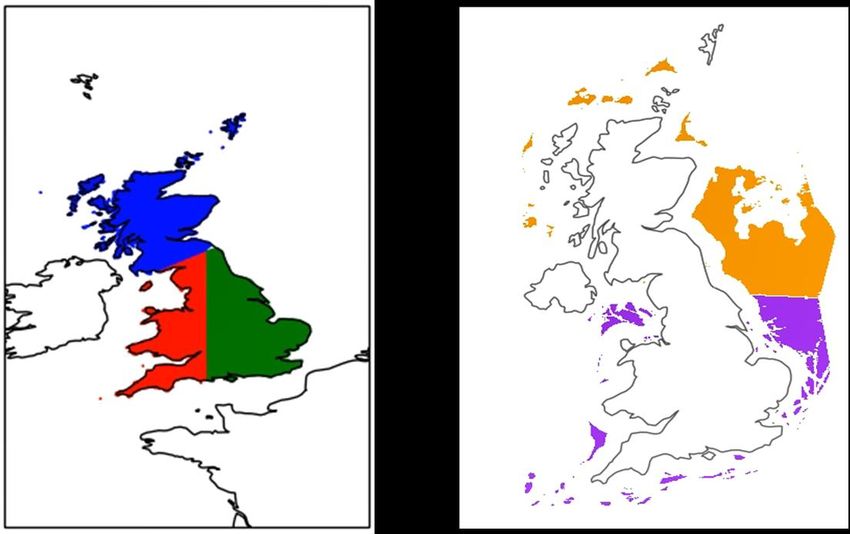
project have been used to calculate the capacity factor in a given grid cell. These 3 turbines
were chosen by Bloomfield et al. (2019) to be representative of type 1, 2 and 3 turbines from
the International Electrotechnical Commission (IEC) wind speed classification respectively
(IEC, 2005). In each land grid cell, the most appropriate turbine (out of these three options) is
chosen, based on the average weather conditions there. Specifically, as in Bloomfield et al.
(2019), it is assumed that all of the turbines within a grid cell are of the same type, and the
selected turbine type is the one that maximises the capacity factor for the 36-year (1979-2014)
mean of the bias corrected 100 m wind speed in that grid cell. Following the continued
guidance from the project advisory group, the off-shore wind power capacity factor is specified
as following the power curve used by National Grid when modelling off-shore turbines
(described in Section 3.2 of nationalgridESO 2019).

Within each grid cell, the wind power capacity factor is then weighted by the potential for
installed wind capacity within that grid cell. The potential for installed wind capacity is based
on the analysis of Price et al. (2018), Moore et al. (2018) and Price et al. (2020). Within these
studies, the potential locations of on-and offshore wind turbines in Great Britain are derived
based on in-depth explorations of technical, social and environmental restrictions. For
example, on-shore restrictions include terrain steepness, distance from housing and the
location of nature conservation areas, while off-shore restrictions include water depth,
shipping routes and the UK government approval of off-shore regions for energy production.

The weighted wind power capacity factors are then aggregated into the defined project regions
for onshore (Figure 1a) and offshore wind (Figure 1b). For onshore wind there are three
regions: Scotland (blue), East England (green) and West England and Wales (red), which
were defined based on the long-term climatology of mean annual 100m wind speed across
the region, calculated from the NEWA data. These are referred to within this report as
‘Onshore North’, ‘Onshore East’ and ‘Onshore West’. Offshore wind has been handled
independently of onshore wind and separated into a north (orange) and south (purple) region
following insights from the project advisory group.

 Page 14 of 79
© Crown copyright 2022, Met Office

Figure 1: (a - Left) Defined project regions for Onshore wind: Scotland (blue), East England (green) and West
England and Wales (red), and (b - Right) Defined project regions for offshore wind: offshore north (orange) and
offshore south (purple).

In summary, the hourly wind power capacity factor in a region is found by multiplying the wind
power capacity factor, in each grid cell within that region, by the potential installed wind
capacity weighting calculated for that grid cell (as a fraction of the total capacity weight in that
region) and aggregating over the region.

To validate the resulting data, daily means of wind power capacity factor for Great Britain were
calculated for each year and plotted against the daily mean of wind power capacity factor for
United Kingdom that were calculated using ERA5 data in phase 2 (Dawkins et al. 2021b). This
validation (Appendix 2) shows good agreement between the datasets across the years. Note
minor discrepancy between the means is expected due to the phase 2 results including results
for Northern Ireland, and small differences in the underlying meteorological data. This confirms
that the hourly wind capacity factors have been calculated successfully in this phase of the
project.

 Estimating solar electricity capacity factor
The method below, as per phase 2, is based on insights from Bloomfield et al. (2019), who
follow a similar approach to Bett and Thornton (2016). Similar to Bloomfield et al. (2019), the
calculation is based on gridded near surface air temperature and incoming surface solar
radiation over land. As in the previous sections of this report, these variables are taken from
the Euro4 hindcast dataset.

 Page 15 of 79
© Crown copyright 2022, Met Office

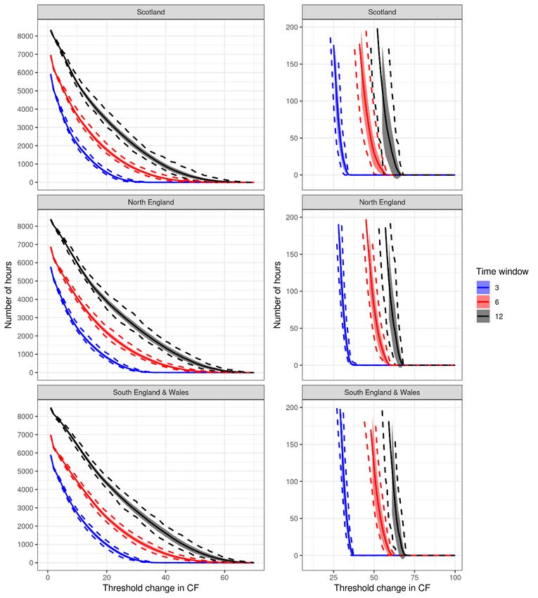
On a given day and within a given land grid cell, the solar power capacity factor, defined as
the proportion of a solar panel’s maximum possible generation produced, is calculated based
on a linear function of the surface temperature and incoming surface solar radiation. This
function first calculates the relative efficiency of the solar panel, η, as a function of surface
temperature at that location and time, T,:

 η(T) = η (1 − ( − )) (1)

where ηr is the photovoltaic panel efficiency evaluated at the reference temperature Tr, and βr
is the fractional decrease of cell efficiency per unit temperature increase. Following Bloomfield
et al. (2019) and Bett and Thornton (2016), the constants in Equation 1 are defined as: ηr=0.9,
Tr=25◦C and βr=0.00042. Here, the temperature at the location of the solar panel, T, is the grid
cell near surface temperature value taken from the ERA5 dataset. The solar power capacity
factor at the given time and location (grid cell) is then calculated as:

 CF = ( ) (2)
 
where G is the incoming surface solar radiation at that location and time, and Gr is the
reference incoming surface solar radiation, set to 1000Wm−2 as in Bloomfield et al. (2019). As
these are linear functions of temperature and solar radiation, solar generation varies linearly
with these meteorological variables. This linear relationship is increasing with solar radiation
and decreasing with temperature.

As in Section 3.1, the solar power capacity factor within each grid cell is then weighted by the
potential for installed solar capacity within that grid cell. The potential for installed wind
capacity is based on the analysis of Price et al. (2018) and as for installed wind capacity, Price
et al. (2018) devise a region within Great Britain, within which solar capacity could be installed,
based on a number of technical, social and environmental restrictions. These include ground
steepness, land use type (e.g. areas of outstanding natural beauty), and policies to protect
wildlife habitats.

The weighted solar power capacity factors are aggregated into the defined project regions
(Figure 2), of which there are three: Scotland (blue), North England (red) and South England
and Wales (green). The regions for solar differ from those used in the onshore wind analysis
as incoming solar radiation has a stronger correlation with latitude rather than longitude,
therefore an east/west split would be of little additional value. As in described in Section 3.1,
the aggregated weighted solar power capacity factors are then scaled by the total region area
capacity to obtain the final hourly solar capacity factor in each region.

 Page 16 of 79
© Crown copyright 2022, Met Office

Figure 2: Defined project regions for solar: Scotland (blue), North England (red) and South England and Wales
 (green).

As described in Section 3.1, a validation was undertaken for each year to compare the daily
means of solar power capacity factor for Great Britain against the daily mean of solar power
capacity factor for United Kingdom calculated using ERA5 data in phase 2. Similarly, the
validation indicated a good agreement between the datasets (Appendix 2).

 Calculating the change in capacity factor over time windows
Using the methods described in Section 3.1 and 3.2, we are able to produce a time series of
hourly capacity factor from 1979-2014 for Great Britain and our defined wind and solar regions.
As in Cannon et al. (2015), a short-duration ramping event for a given region, is quantified as
the maximum change in capacity factor, within a given time window. The time windows
explored are those used by Cannon et al. (2015): 1 hour, 3 hours, 6 hours, 12 hours and 24
hours. For a given time window e.g., 3 hours and region e.g. Scotland, the number of times
this ‘maximum capacity factor change’ surpasses a particular change threshold can be
calculated. As in Cannon et al. (2015), the average number of ramping events per year that
surpass each change threshold of interest for a given time window can then be determined.
This allows us to compare our analysis of ramping events to that of Cannon et al. (2015), and
provides insights into the frequency of different size ramping events in any suitable
meteorological dataset.

 Page 17 of 79
© Crown copyright 2022, Met Office

An important thing to note is this calculation is carried out using rolling time windows, moving
through the hourly timeseries data from 1979-2014. The maximum change in capacity factor
could occur at any point during a given time window, and therefore where two-time windows
may overlap, there is the potential for repeated data points where one ramping event is double
counted. For example, as shown in Figure 3 below, these two 3-hour time windows (indicated
in black) have the same maximum change in capacity factor but are counted as two ramping
events. The repeated data points will need to be handled during the extreme value analysis
(EVA).

 Figure 3: Schematic to show two overlapping 3-hour time windows (black) over a timeseries (pink) which would
 have the same maximum change in capacity factor.

In addition as mentioned in Section 3.1 the reinitialisation of the model underlying the wind
speed data may result in spurious ramps being identified. For this reason, if a 1, 2 or 3 hour
window contains such a model reinitialisation, then it is excluded from the further analysis so
that conclusions are based upon plausible meteorological conditions rather than model
features. For longer time windows the reinitialisation was found to not make material difference
to the ramps identified.

Finally, as described in Section 3, the capacity factor defines, for a given time period, the ratio
of actual generation compared to the maximum potential generation. As a ratio, the capacity
factor is unitless and is usually given as a number between 0 and 1. For the presentation of
results in this report, the capacity factor is given as a number between 0 and 100 to allow for
the replication and comparison of analysis carried out in Cannon et al. (2015). This should not
be confused as a percentage change in capacity factor. For example, within this report, a
change in capacity factor of 50 is equivalent to an absolute change of 0.5 (i.e. a capacity factor
dropping from 0.8 to 0.3), not a 50% change (e.g. a capacity factor decrease from 0.8 to 0.4).

 Extreme Value Analysis
For each time window and region, an empirical EVA is carried out to contextualise the
extremity of ramping events, particularly focusing on the most extreme events. This empirical
(I.e., based on the observed data record only) EVA identifies the observed return period
(number of years in between events) of ramping events of a given return level (extremity of

 Page 18 of 79
© Crown copyright 2022, Met Office

‘change in CF’). For example, allowing us to identify that, for wind ramping events in 3-hour
time-windows in the Onshore North region, a change in CF of 70 occurs on average once
every 10 years.

For each time window and region, the empirical return period (in years) of each ramp ‘event’
(I.e., the maximum change in CF in each overlapping time window) is estimated empirically
by firstly ranking all events in ascending order, equivalent to calculating the event percentile.
This calculates the event frequency in terms of events, for example, as described in phase 2a
(Dawkins and Rushby 2021), the 50th percentile event (ranked exactly in the middle) is the
event expected to occur once every 2 events. These percentiles are then scaled by the
number of years and the number of events in the data record, to give a return period in terms
of years (rather than events). For example, we have 36 years of data (1979-2014) and there
are 315,549 overlapping 3-hour time windows in 36 years (I.e. 315,549 events), hence the 1
in 2 events 3-hour time window event (the 50th percentile or middle ranked) is the 1 in 36/(0.5
x 315,549) year event (I.e., the 1 in 0.0023-year event, hence expected to occur 4382 times
per year). Similarly, here, the 99.99th percentile event is the 36/(0.0001 x 315,549) year event
(I.e. the 1 in 1.14-year event, hence expected to occur approximately once per year).

As noted in Section 3.3, the way in which the ramping events are characterised leads to some
events being double counted, and hence the events being temporally correlated. This can lead
to a misrepresentation of the return period of events (Coles, 2001). To overcome this, the
events are ‘de-clustered’ before the return periods are estimated using the approach described
above. De-clustering is achieved by firstly defining a high threshold, then each time this high
threshold is exceeded for multiple events in a row, only the most extreme event is retained.
This ensures the same ramping event is not represented multiple times within the extremes of
the dataset, and hence the EVA. Here, the data for each time window and region is de-
clustered using a 95th percentile threshold.

This method is used to identify the 1 in 2, 5, 10, 20 and 30-year return period wind and solar
ramping events for each region and time window combination. This allows for return level
curves to the plotted for each region and time window, for comparison. Examples of such
events are also selected from the Euro4 data record, presented in tables, and as timeseries
plots for context (see Sections 4.1.3 and 4.2.2).

 Page 19 of 79
© Crown copyright 2022, Met Office

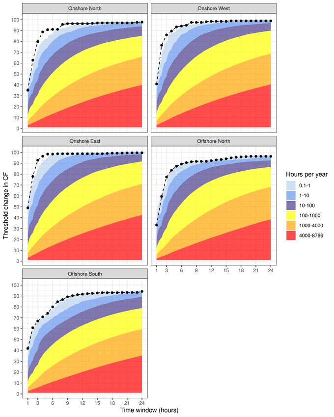
4 Results

 Wind
In this section we present the analysis of historical observed wind ramping events from the
Euro4 data record. This analysis follows closely with the approach taken by Cannon et al.
(2015), with equivalent plots produced. Firstly, this is done for GB as a whole for comparison
with Cannon et al. (2015), and secondly for each of the 5 wind regions separately.

4.1.1 Maximum change in capacity factor in Great Britain over various time windows

Figure 4, equivalent to Figure 9(c) in Cannon et al. (2015), shows, for a given time window on
the x-axis, the number of times in an average year that the maximum change in capacity factor
(hereafter referred to as ΔCF) surpasses a particular change threshold (y-axis) in Great
Britain. For example, in an average year, the maximum change in capacity factor during a 6-
hour time window will surpass at least 10 between 4000–8767 hours per year compared to
surpassing at least 47 between 10-100 hours per year. The most extreme ramping event
identified in Great Britain across the 36-year time series (indicated by the dashed line) during
a 6-hour time window was a ΔCF of 68.

 Page 20 of 79
© Crown copyright 2022, Met Office

Figure 4: The frequency of hours, in an average year, for which there is a subsequent ramp in generation of at
least ΔCF (y-axis) within the given time window (x-axis) for Great Britain. The dashed lines mark the most extreme
events in the 36-year time series (1979-2014). ΔCF = maximum change in capacity factor observed in a given time
window.

Cannon et al. (2015), from which this method was based on, explored the frequency of rapid
change wind ramping events in the UK from 1980-2012 and noted the following key
observations:

 • As the threshold change increases or the time window decreases, the definition of
 a ramp becomes more stringent and therefore ramping becomes rarer.
 • In correspondence to the transition time of a typical low pressure (cyclonic) weather
 system over the UK, the most extreme changes in maximum capacity factor
 change (indicated by the dashed line) increases rapidly with the time window up to
 around 9-12 hours, after which it plateaus.

The results presented are consistent with those produced by Cannon et al. (2015) and the
observations outlined above, although the observed changes in capacity factor are generally
10% higher here. This is hypothesised to be due to the difference in the wind power curves

 Page 21 of 79
© Crown copyright 2022, Met Office

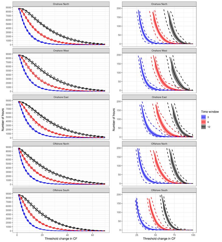
used, with the power curve in the Cannon et al. (2015) paper plateauing at a 90% capacity
factor, and the different spatial distribution of wind turbines across Great Britain.

Cannon et al. (2015) found that the most extreme changes in capacity factor (the dashed line)
increase rapidly with time window to around 12 hours, after which it plateaus. They associate
this with the transition time of a typical low pressure (cyclonic) weather system over the UK.
Figure 4 shows a more gradual increase in the most extreme changes in capacity factor with
time window in comparison to Cannon et al. (2015), with a later plateau at closer to 15 hours.
It is suspected that this difference is largely reflecting the difference in region size over which
the capacity factor is aggregated, with this work undertaken over a wider GB domain, capturing
more offshore wind regions. Therefore, the transition time of weather system across GB is
expected to take longer to move across the larger domain. Furthermore, it is also anticipated
that the increased spatial resolution of the Euro4 hindcast meteorological data is more
accurately representing the meteorological extremes in the shorter time windows, compared
to MERRA reanalysis data (50km) used in Cannon et al. (2015), and could explain the
additional variability captured in the most extreme changes in capacity factor.

4.1.2 Maximum change in capacity factor across defined regions over various time
 windows

Figure 5, equivalent to Figure 9(c) in Cannon et al. (2015), shows, for a given time window on
the x-axis, the number of times in an average year that the maximum change in capacity factor
change (ΔCF) surpasses a particular change threshold (y-axis) for each of the defined regions
for onshore and offshore wind. Looking at ‘Offshore South’ as an example (Figure 5, third row,
left), the most extreme ΔCF observed in a 1-hour time window in the last 36 years is 42 (black
star). For the same region, in an average year, the ΔCF surpassing at least 28 was observed
less than once a year during a 1-hour time window compared to between 4000-8766 times
during a 24-hour period.

There are some subtle differences in the regional plots shown in Figure 5. For example,
‘Onshore East’ frequently experiences larger ΔCF during the shorter time windows, indicated
by the steep gradient of the dashed line between the 1–6-hour time windows - the maximum
ΔCF seen in a 6-hour time window is approximately the same as that of a 24-hour window In
terms of wind ramping events observed over the 36-year timeseries, ‘Onshore East’ reaches
the plateau of threshold change by the 6-hour time window, in comparison to the 9-hour time-
window for ‘Onshore North’ and ‘Onshore West’. In an average year, both offshore regions
are observed to have smaller, less frequent ramps during the shorter time windows compared
to the onshore regions, indicated by the gentler increasing slope of the dashed line through

 Page 22 of 79
© Crown copyright 2022, Met Office

the time-windows. Further, of all the regions, ‘Offshore North’ has the smallest observed
maximum change in capacity factor (ΔCF = 33) during a 1-hour time window across the 36-
year timeseries.

Figure 5: The frequency of hours for which there is a subsequent ramp in generation of at least ΔCF (y-axis)
within the given time window (x-axis) for the defined regions of onshore and offshore wind. The dashed lines
mark the most extreme events in the 36-year time series (1979-2014).

 Page 23 of 79
© Crown copyright 2022, Met Office

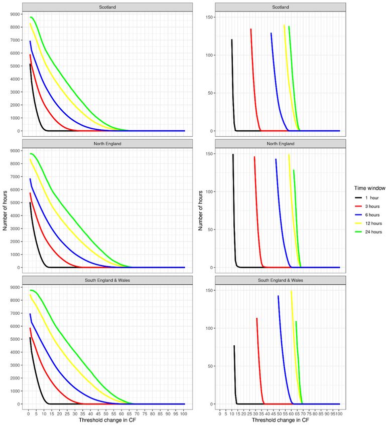
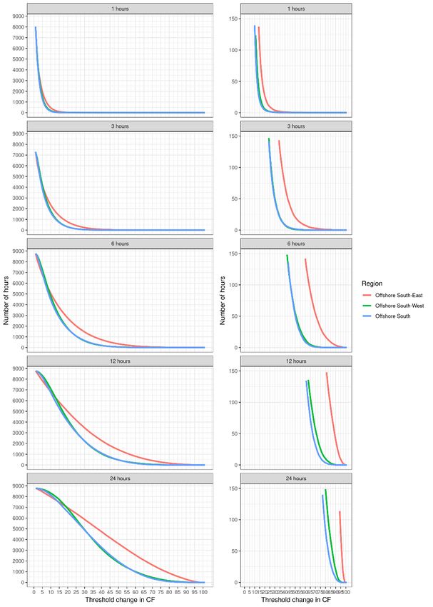
Figure 6, equivalent to Figure 8(c) and (f) in Cannon et al. (2015) shows, for each region (one
per row) and time window (coloured lines), the number of times in an average year (y-axis)
that a ramp event is observed reaching or exceeding a threshold of ΔCF (x-axis). Each line
on the plot represents a different time window (1-, 3-, 6-, 12- and 24- hour time windows) with
a row per a defined region – identified in the top grey bar. The right-hand panel presents an
exploration of the less frequent ramping events for each region i.e., focusing on events
reaching a threshold change less than 150 times (number of hours) in an average year. For
example, in the case of ‘Onshore North’, Figure 5 indicates that, in an average year, the
maximum change in capacity factor surpassing at least 40 was observed between 10-100
times during a 3-hour time window. The left-hand panel of Figure 6 below suggests that, for
the same region and time window there is a plateau towards 0 occurrences for all threshold
changes above ΔCF = 25. Using the right-hand panel of Figure 6, it is possible to explore
these lower frequency events in higher resolution and read from the plot that, during an
average year, ΔCF >= 40 in a 3-hour window occurs approximately 20 times in the ‘Onshore
North’ region (highlighted by the red star).

Figure 6 highlights that, in an average year, the number of times a ramp reaches a threshold
of capacity factor change decreases as that threshold increases i.e., the higher thresholds are
surpassed left often. A common feature across all the regions is that the maximum change in
capacity factor (ΔCF) is larger during the bigger time windows, which is consistent with the
findings of Cannon et al. (2015). This is particularly evident when focusing on the less frequent
ramp events occurring in an average year, highlighted in the right-hand panel of Figure 6.
Comparing the 1-, 6- and 24-hour time windows for ‘Onshore West’, the threshold for
maximum change in capacity factor observed around 125 times in an average year, is around
15, 50 and 90, respectively. As a similar observation can be made across all of the regions,
the national electricity system may be vulnerable should these larger changes occur
simultaneously within the longer time window. Hence, to allow energy modellers to explore
this potential vulnerability, the final data set of short duration events will contain spatial fields
of meteorological data covering all of GB and the offshore region for the full time slice of the
passage of weather systems.

 Page 24 of 79
© Crown copyright 2022, Met Office

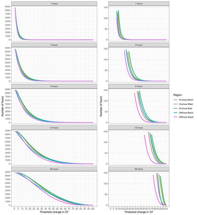
Figure 6: The number of hours in an average year (y-axis) that a ramp event is observed reaching or exceeding a
threshold of ΔCF (x-axis). Each line on the plot represents a different time window (1-, 3-, 6-, 12- and 24- hour
time windows) with a row per a defined region – identified in the top grey bar. The right-hand panel presents an
exploration of the less frequent ramping events for each region i.e., focusing on events reaching a threshold
change less than 150 times (number of hours) in an average year.

Similarly, Figure 7 shows, for each time window (one per row) and region (coloured lines), the
number of times in an average year (y-axis) that a ramp event reaches or exceeds a threshold
of capacity factor change (x-axis). The uniform shape of the different coloured lines indicate
that the different regions are relatively consistent in their fluctuations of ΔCF across the various
time windows. There is also a slight indication that the two offshore regions have a smaller
magnitude in fluctuations compared to onshore regions, particularly offshore south, indicated

 Page 25 of 79
© Crown copyright 2022, Met Office

by the leftward shift of the pink lines in Figure 7. It is hypothesised that the offshore regions
experience smaller fluctuations as a result of the greater spatial distribution of turbines over a
wider area, in comparison to the onshore regions. This means that as a low-pressure weather
system moves across, it is less likely for the whole region to be disrupted simultaneously, with
non-affected areas balancing those experiencing fluctuations (in the sense of averaging the
capacity factor change over the region). Of the two offshore regions, Offshore South is the
most widely distributed, with turbine capacity spanning off the east and west coasts of
southern England. Furthermore, when observing the capacity factor maps (not shown here),
the overall capacity of Offshore South is less, which means theoretically there is less potential
magnitude for change to start with. These findings, whilst not taking account of the flexibility
offered by storage, or other implications governing turbine locations, support the results of
Drew et al. (2017) that favour an increased spatial distribution across Great Britain, both
onshore and offshore, to improve energy system resilience.

 Page 26 of 79
© Crown copyright 2022, Met Office

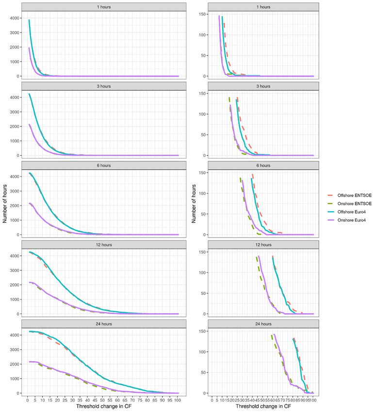
Figure 7: The number of hours in an average year (y-axis) that a ramp event is observed reaching or exceeding a
threshold of ΔCF (x-axis). Each line on the plot represents a different defined region with a row per a time window
– identified in the top grey bar. The right-hand panel presents an exploration of the less frequent ramping events
for each time window i.e., focusing on events reaching a threshold change less than 150 times (number of hours)
in an average year.

Plots to explore the interannual and seasonal variability of wind ramping events in an average
year (equivalent to Figure 11 and 12 (c) and (f) in Cannon et al. (2015)) were also produced
for the different regions, and are Appendix 3 and 4, respectively.

Cannon et al. (2015) observe large interannual variability, which is particularly true for the
most extreme events. Whilst the full range plot in the left-hand panel of Appendix 3 appears
to present little year-to-year variability for any time window or region, the right-hand panel

 Page 27 of 79
© Crown copyright 2022, Met Office

presenting the least frequent events does highlight a greater magnitude of variability in the
most extreme events, as observed in Cannon et al. (2015). Onshore East and Onshore West
appear to have the most variability of the regions, particularly so in the most extreme events
observed in any one year where thresholds changes in capacity factor are surpassed less
than 100 hours per year. The deviation away from the mean is greatest in events observed
less than 50 times, which is a common feature across the regions, although to varying
magnitudes. A consideration for the resilience of future systems may be that even small
differences in the observed year-to-year variability (i.e., a small number of extreme ramping
events with ΔCF that deviate from the mean) could multiply up in significance if there is an
increased capacity of wind installed.

Appendix 4 shows that the most frequent but small ΔCF appear to occur most often in summer
and spring with these seasonal lines falling above the average season and autumn and winter
falling on or below, which holds across the regions for ΔCF up to between 20-30. Cannon et
al. (2015) note that the mean frequency of ramps varies seasonally, noting that there are many
more extreme ramps in winter than in summer, likely due to the cyclonic activity over the UK
in winter. This is consistent with the findings observed in the right-hand panel of Appendix 4,
although observed to a lesser extent in the ‘Onshore North’ (Scotland) region where there is
little seasonal variability, indicated by the overlapping of the different season lines and minimal
deviation from the average season. This could probably be related to orographic impact on
wind, that means wind speed volatility and variability is greater across land in Scotland in the
summer compared to the southern regions which have less highland areas proportional to the
region size. The seasonal variability for ‘Offshore South’ tightens (I.e., less difference between
seasons) as ΔCF surpasses the 80 threshold. Comparatively, the seasonal distribution of
‘Offshore North’, ‘Onshore East’ and ‘Onshore West’ narrows closer towards the least frequent
events, surpassing the 90 threshold of change. Interestingly, Cannon et al. (2015) observe
little seasonal variability between summer and winter in the very most extreme ΔCF events for
Great Britain, which appears to be true for this analysis also.

4.1.3 Return periods and return levels of extreme events

Figure 8 presents the results of the empirical extreme value analysis, carried out to calculate
the return period (‘expected’ number of years in between events) of wind ramping events of a
given return level (extremity of ‘change in CF’). The left-hand panel presents the return period
(x-axis) and return level (y-axis) for a time window (each coloured line) within a defined region
(each plot). For example, in the ‘Offshore South’ region, a 1 in 10-year event has a return level

 Page 28 of 79
© Crown copyright 2022, Met Office