Analysis of a Dryline during IHOP: Implications for Convection Initiation
←
→
Page content transcription
If your browser does not render page correctly, please read the page content below
912                                         MONTHLY WEATHER REVIEW                                                             VOLUME 137

          Analysis of a Dryline during IHOP: Implications for Convection Initiation

                                                    ROGER M. WAKIMOTO
                                   National Center for Atmospheric Research, Boulder, Colorado

                                                     HANNE V. MURPHEY
         Department of Atmospheric and Oceanic Sciences, University of California, Los Angeles, Los Angeles, California

                                 (Manuscript received 6 March 2008, in final form 29 August 2008)

                                                             ABSTRACT

              A detailed analysis of a dryline that formed on 22 May 2002 during the International H2O Project (IHOP) is
            presented. The dryline was classified as a null case since air parcels lifted over the convergence boundary
            were unable to reach the level of free convection preventing thunderstorms from forming. A secondary
            dryline associated with a distinct moisture discontinuity developed to the west of the primary dryline. The
            primary dryline exhibited substantial along-frontal variability owing to the presence of misocyclones. This
            nonlinear pattern resembled the precipitation core/gap structure associated with cold fronts during one of the
            analysis times although the misocyclones were positioned within the gap regions. Radar refractivity has been
            recently shown to accurately retrieve the low-level moisture fields within the convective boundary layer;
            however, its use in forecasting the initiation of convection has been restricted to qualitative interpretations.
            This study introduces the total derivative of radar refractivity as a quantitative parameter that may improve
            nowcasts of convection. Although no storms developed on this day, there was a tendency for maxima of the
            total derivative to be near regions where cumulus clouds were developing near a convergence boundary.

1. Introduction                                                      storms (80%) developed near boundary-layer conver-
                                                                     gence zones. In spite of these major findings, it is also
  One of the major challenges during the summer
                                                                     known that the presence of a prominent convergence
months is predicting the initiation of deep, moist con-
                                                                     line is not a sufficient condition for convection to de-
vection (Olsen et al. 1995; Fritsch and Carbone 2004).
                                                                     velop (e.g., Rotunno et al. 1988; Stensrud and Maddox
Forecasters often have difficulty assessing, under weak
synoptically forced conditions, the potential of rising              1988; Crook 1996; Ziegler and Rasmussen 1998; Crook
parcels of air to reach the level of free convection (LFC)           and Klemp 2000; Richter and Bosart 2002; Cai et al.
and then maintaining positive buoyancy as they pass this             2006; Markowski et al. 2006).
level. Improvements in these short-term forecasts, how-                 Stensrud and Maddox (1988), Richter and Bosart
ever, resulted when organized lines of convergence that              (2002), and Cai et al. (2006) have shown that larger-scale
form in the boundary layer were successfully detected                descent can prevent convection initiation even when large
using remote sensing techniques (e.g., Purdom 1976,                  convective available potential energy (CAPE) and con-
1982; Wilson and Schreiber 1986; Wilson and Mueller                  ditionally unstable environments exist. Rotunno et al.
1993; Wilson et al. 1998). Purdom (1982) provided evi-               (1988) have proposed that the balance of horizontal
dence that 93% of the storms forming over the south-                 vorticity generated by the ambient low-level shear with
eastern United States were associated with arc clouds                the baroclinically produced vorticity owing to the cold
that were associated with convergence lines. Wilson and              pool to the rear of a boundary can alter the orienta-
Schreiber (1986) showed that a majority of thunder-                  tion of the updraft. Vertically erect updrafts might be
                                                                     more likely to produce deep convection. Ziegler and
                                                                     Rasmussen (1998) have suggested that air parcels that
  Corresponding author address: Roger M. Wakimoto, NCAR/
                                                                     are lifted from the boundary layer must reach the lifted
EOL, P.O. Box 3000, Boulder, CO 80307.                               condensation level (LCL) and the LFC prior to leaving
E-mail: wakimoto@ucar.edu                                            the mesoscale updraft to form deep convection.

DOI: 10.1175/2008MWR2584.1

Ó 2009 American Meteorological Society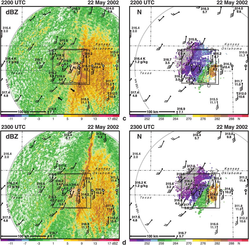
MARCH 2009                               WAKIMOTO AND MURPHEY                                                        913

   Additional challenges have been suggested based on            Another aspect of this study is to examine further the
results from numerical simulations. Lee et al. (1991) and     utility of radar refractivity in providing thermodynamic
Crook (1996) have shown that relatively small changes         information that can be used to improve convective
in mixing ratio (e.g., 1 g kg21) can have a significant       forecasts. Radar estimates of refractivity can be derived
effect on the developing convection. These findings are       by measuring the apparent fluctuations in the range of
challenging to address since comprehensive measure-           fixed ground targets. Variations of refractivity are pri-
ments of moisture have been difficult to collect in field     marily owing to changes in water vapor under typical
studies. Moreover, variations of moisture over distances      warm summertime temperatures (Fabry et al. 1997;
of only a few kilometers, as suggested by the modeling        Fabry 2004, 2006). Weckwerth et al. (2005) have shown
studies, have been shown to commonly occur within the         the excellent agreement between radar refractivity and
convective boundary layer (e.g., Weckwerth et al. 1996;       surface moisture gradients; however, most past studies
Weckwerth 2000; Murphey et al. 2006).                         have used refractivity in a qualitative manner for im-
   The present study focuses on a dryline that developed      proving forecasts (e.g., Cai et al. 2006; Demoz et al.
on 22 May 2002 during the International H2O Project           2006; Fabry 2006; Buban et al. 2007).
(IHOP; Weckwerth et al. 2004). The dryline is a con-             Section 2 discusses Electra Doppler radar (ELDORA)
vergence line that frequently forms over the south-           and S-band dual-polarization Doppler radar (S-Pol),
western United States as hot dry air from the Mexican         which are two of the primary platforms used in this
plateau collides with moist air flowing northward from        study. Surface and ground-based radar analyses are
the Gulf of Mexico. Its association with deep (severe)        presented in section 3. Vertical cross sections based on a
convection has been noted for a number of years (e.g.,        series of soundings through the dryline and an airborne
Rhea 1966; Schaefer 1974, 1986; Bluestein and Parker          Doppler radar analysis are shown in sections 4 and 5,
1993). The dryline on 22 May was well sampled by a            respectively. A summary and conclusions are presented
number of platforms during IHOP and has been ex-              in section 6.
tensively examined (Demoz et al. 2006; Weiss et al.
2006; Buban et al. 2007). The boundary that developed
on this day also generated interest since it was a null
                                                              2. ELDORA and S-Pol
case; that is, a boundary that was not associated with the
initiation of convection.                                       One of the primary platforms used in the study is
   A unique aspect of this study is an airborne Doppler       a 3-cm airborne Doppler radar (ELDORA) operated
radar that was used to collect kinematic data along this      by the National Center for Atmospheric Research
frontlike boundary. The aircraft flew a box pattern           (NCAR) and flown on board a Naval Research Labo-
around the dryline with the along-boundary legs ;100          ratory (NRL) P-3. ELDORA is equipped with two an-
km long. These long legs allowed for an accurate as-          tennae that scan fore and aft of the normal to the air-
sessment of both the along-frontal variability and the        craft. Data collected by the radar can be synthesized
mean characteristics of the dryline. Detailed observa-        into a dual-Doppler windfield using the fore–aft scan-
tional studies have already shown that substantial vari-      ning technique (FAST; Jorgensen et al. 1996). Critical
ability along convergence boundaries can exist (e.g.,         to this study was ELDORA’s ability to detect echoes
Kingsmill 1995; Friedrich et al. 2005; Arnott et al. 2006;    and Doppler velocities within the clear air (Wakimoto
Markowski et al. 2006; Murphey et al. 2006). Demoz            et al. 1996). Convergence boundaries often appear as
et al. (2006) provided high-temporal resolution data of       radar-detectable thin lines even in the absence of pre-
the vertical structure of this dryline but it was primarily   cipitation particles (e.g., Wilson and Schreiber 1986).
focused on measurements made from a single site.              Research flight plans required the P-3 to fly at low levels
Weiss et al. (2006) analyzed the vertical structure of the    [;400 m above ground level (AGL); hereafter, all
dryline with unprecedented detail but only in a plane         heights are AGL except where indicated] and parallel
normal to the boundary. Buban et al. (2007) examined a        to the thin lines. The thin line was positioned within 2–3
30 km 3 30 km section of the dryline using ground-            km from the aircraft and resulted in a flight track that
based Doppler radars. Their study was largely based on        resembled a box-type pattern ;100 km long. The radar
a Lagrangian analysis of thermodynamic variables. The         scanning parameters used during IHOP are shown in
analysis depends on advecting in situ data collected          Table 1 and a discussion of the radar methodology is
along one-dimensional transects using parcel trajecto-        presented in the appendix. For more information re-
ries derived from the multi-Doppler radar analysis.           garding ELDORA’s hardware and design, the inter-
Local conservation following the motion is also as-           ested reader is referred to Hildebrand et al. (1994,
sumed (Ziegler et al. 2007).                                  1996).
914                                      MONTHLY WEATHER REVIEW                                                     VOLUME 137

            TABLE 1. ELDORA scanning mode.

Antenna rotation rate (8 s21)                         75
Number of samples                                     60
Pulse repetition frequency (PRF) (Hz)               3000
Gate length (m)                                      110
Sweep-angle resolution (8)                             1.5
Along-track resolution (m)                          ;600
Maximum range (km)                                    50
Maximum unambiguous velocities (m s21)               623.6

   Measurements of radar refractivity during IHOP were
obtained using S-Pol, an S-band multiparameter radar
(Lutz et al. 1995). Refractivity values can be derived by
identifying ground targets (e.g., towers, buildings, poles)
that surround the radar site and quantifying the small
variations in the return phase from stationary targets
caused by changes in the index of refraction in the in-
tervening atmosphere (Fabry et al. 1997; Fabry 2004).
High correlation between radar refractivity and refrac-
tivity calculated from low-flying aircraft and surface
mesonets was shown by Weckwerth et al. (2005). Buban
                                                                 FIG. 1. Surface analysis for 2100 UTC 22 May 2002. Isobars (gray
et al. (2007) showed close agreement between two-             lines) and mixing ratio (black lines) are shown. Locations of the
dimensional water vapor fields derived from radar re-         fronts and a dryline are indicated on the analysis. Values of mixing
fractivity with analogous fields calculated from in situ      ratio greater than 12 g kg21 are shaded gray. Wind vectors are
data. The maximum range for retrieved estimates of            plotted using the following notation: barb 5 5 m s21, half barb 5
                                                              2.5 m s21.
refractivity from S-Pol data collected during IHOP was
between 40 and 60 km.
                                                              highlighted by the black arrows in Fig. 3a. The middle
                                                              fine line was located on the eastern edge of a dry air mass
3. Surface and radar analyses
                                                              as shown by the mixing ratio values and the low values of
   An upper-level trough was situated over the western        radar refractivity (N values , 255). The eastern fine line
United States at the 500-mb level (not shown). At the         is diffuse; however, it denotes the incipient stages of the
surface, there was a cyclone over southeastern Colorado       primary dryline that formed on this day. The western fine
resulting in southerly flow over the south-central United     line is not a focus in this study and becomes less defined
States (Fig. 1). These conditions are typical for a well-     with time. An enlargement of Fig. 3a is shown in Fig. 4a.
defined dryline to develop (e.g., Schultz et al. 2007). The   There is a drop in mixing ratio (.6 g kg21) from just east
dryline is located at the leading edge of a gradient of       of S-Pol to the western edge of the region shown in Fig.
mixing ratio and a convergence boundary in the surface        4a. This horizontal gradient of moisture is also apparent
wind-field analysis at 2100 UTC over the Oklahoma and         in the analysis of N (color plot and isopleths).
Texas panhandles (Fig. 1).                                       Surface confluence across the dryline increases at
   Surface analyses at 2000, 2100, 2200, and 2300 UTC         2100 UTC as the winds began to back within the moist
superimposed on visible satellite images are presented        air (Fig. 2b). The moisture discontinuity associated with
in Fig. 2. A dryline in Fig. 2a was determined by a           the primary dryline also increases in response to this
combination of the surface mixing ratios and also             enhanced confluence based on the isopleths of N (Fig. 4b).
placing the boundary near the western edge of the cu-         Another boundary (denoted by a dashed line) has been
mulus cloud field that was apparent in the satellite im-      drawn on the analysis at 2100 UTC (Fig. 2b) and is in-
age. The beginning of the flight track flown by the P-3 is    dicative of the formative stages of a second dryline (also
shown by the dotted line (Fig. 2a). This westbound flight     noted by Buban et al. 2007). At this time, the secondary
leg was intended to provide an initial survey of the near     dryline is accompanied by a weak horizontal gradient of
surface conditions in order to identify any convergence       moisture in the N-field in the western section in Fig. 4b.
boundaries in the region. There were several fine lines       Miao and Geerts (2007), however, showed that no
(i.e., enhanced lines of radar reflectivity) seen in the      measurable virtual potential temperature gradient existed
surveillance scan of S-Pol radar reflectivity that are        across the secondary boundary. Weiss et al. (2006) also
MARCH 2009 WAKIMOTO AND MURPHEY 915
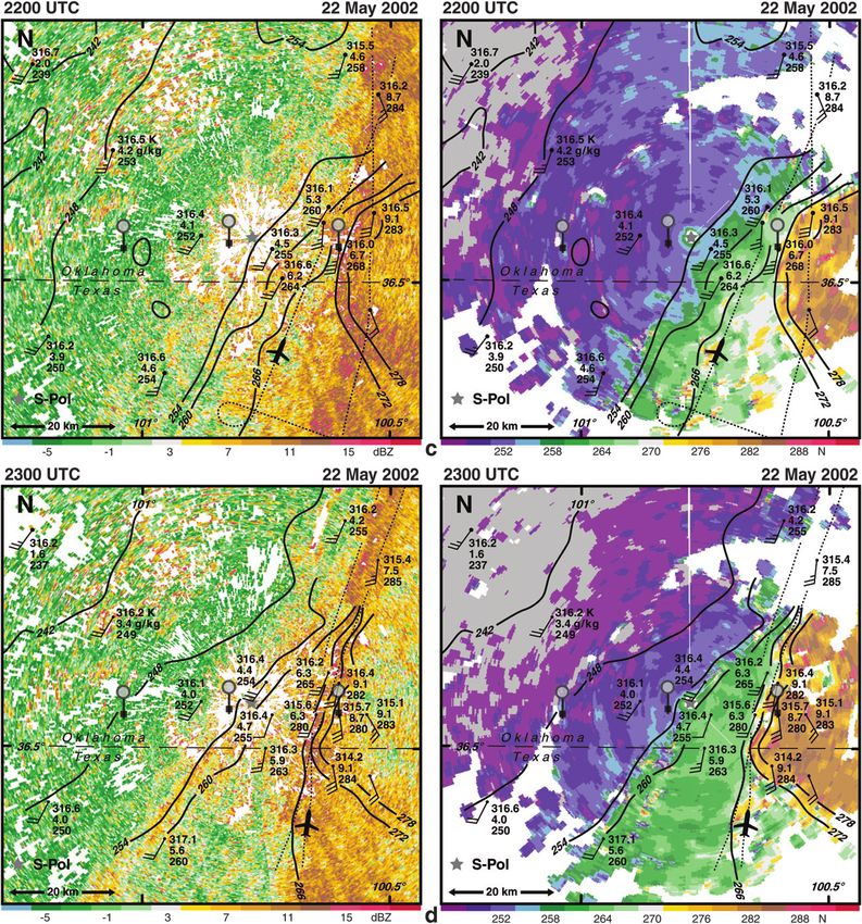
FIG. 2. Surface analysis for (a) 2000, (b) 2100, (c) 2200, and (d) 2300 UTC 22 May 2002 superimposed onto visible
satellite images. Virtual potential temperature (K) and mixing ratio values (g kg21) are plotted. Primary and sec-
ondary drylines are shown on the analyses. Sounding locations are shown on the image at 2200 and 2300 UTC. The
track of the P-3 is shown by the dotted line. The small box represents the location of the dual-Doppler analysis shown
in Fig. 8. Wind vectors are plotted using the following notation: barb 5 5 m s21, half barb 5 2.5 m s21.
estimated that the secondary dryline formed around this errors are transient and not predictable based on known
time. The existence of double drylines has been well doc- meteorological features (Weckwerth et al. 2005; Buban
umented in the literature (e.g., Hane et al. 1997; Crawford et al. 2007).
and Bluestein 1997; Hane et al. 2001). It should be noted Cumulus clouds were prevalent throughout the tri-
that the drier air that is suggested by the low refractiv- angular region bounded by the two drylines at 2200
ity values in the southeast corner of Fig. 4b is believed UTC (Fig. 2c). The fine line associated with the primary
to be in error (e.g., Buban et al. 2007; also compare this dryline has become more prominent (Fig. 3c; note the
plot with the one shown in Fig. 4a). In situ data collected eastern arrow) and in the enlargement (Fig. 4c), which is
at flight level (to be discussed later) reveals that the consistent with the presence of strong surface conver-
southeastern air mass is still moist. Possible reasons for gence (Wilson et al. 1994). Dry air now extends much
these errors include nonstationary targets and swaying further to the east by comparing the positions of the
vegetation (Fabry 2004; Weckwerth et al. 2005). These N 5 254 isopleth at 2100 and 2200 UTC (Figs. 4b,c). The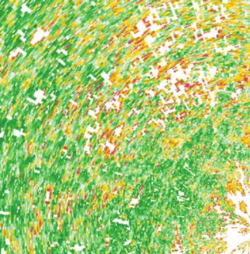
916                                            MONTHLY WEATHER REVIEW                                                            VOLUME 137

   FIG. 3. Surface observations for (a) 2000, (b) 2100, (c) 2200, and (d) 2300 UTC 22 May 2002 superimposed onto (left) radar reflectivity
and (right) radar refractivity images. Virtual potential temperature (K) and mixing ratio values (g kg21) are plotted. The track of the P-3
is shown by the dotted line. The black arrows in (a) and (b) denote the positions of three fine lines in radar reflectivity. Sounding locations
are shown on the plots at 2200 and 2300 UTC. The region denoted by the gray square is enlarged in Fig. 4. The black rectangle at 2200 and
2300 UTC represent the location of the dual-Doppler analysis shown in Fig. 8. Wind vectors are plotted using the following notation: barb 5
5 m s21, half barb 5 2.5 m s21. Color scales for dBZ and N values are shown. Gray areas for refractivity denote values of N less than 245.

eastern edge of this dry air is the location of the sec-                    The cumulus cloud activity between the two drylines
ondary dryline and can be identified in the reflectivity                 is more prominent in the satellite imagery at 2300 UTC
pattern as a developing fine line (the western arrow in                  (Fig. 2d). In addition, the fine lines associated with the
Fig. 3c). The P-3 aircraft was in the early stages of flying             primary and secondary drylines are easily identifiable in
a box pattern around the primary dryline as shown by                     the S-Pol surveillance scans (Figs. 3d, 4d). The inter-
the dotted line in Fig. 4c (also shown in Figs. 2c, 3c).                 section of the drylines, which resembles an inverted
MARCH 2009                              WAKIMOTO AND MURPHEY                                                        917

                                                   FIG. 3. (Continued )

V-shape, is located ;30 km northeast of S-Pol and is         dryline has regressed by ;20 km at this time (Fig. 4e).
shown in the refractivity analysis where the two hori-       As a result, the intersection point of the two drylines has
zontal gradients of the N-field merge (Fig. 4d). Further     moved farther to the north.
confirmation that the dry air located in the southeastern
section of the refractivity field in Fig. 4d is erroneous
                                                             4. Vertical cross section based on sounding data
was provided by the in situ data collected at flight level
by the P-3. The flight-level data collected east of the        A series of dropsondes deployed by a jet flying at
boundary shown in the figure revealed moist air in this      ;500 mb between 2215 and 2233 UTC was combined
region (not shown). The primary dryline regresses by a       with three balloon soundings released at 2150, 2235, and
few kilometers by 0000 UTC; however, the secondary           2247 UTC to produce a vertical cross section oriented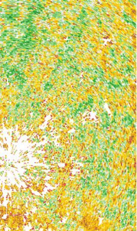
918                                           MONTHLY WEATHER REVIEW                                                           VOLUME 137

   FIG. 4. Surface analysis for (a) 2000, (b) 2100, (c) 2200, (d) 2300 UTC 22 May 2002 and (e) 0000 UTC 23 May 2002 superimposed onto
(left) radar reflectivity and (right) radar refractivity images. Black lines superimposed on both plots are contour values of N. The track of
the P-3 is shown by the dotted line. Virtual potential temperature (K), mixing ratio values (g kg21), and radar refractivity (N) are plotted.
The location of S-Pol is shown by the gray star. The location of the analysis region is shown by the gray box in Fig. 3. Wind vectors are
plotted using the following notation: barb 5 5 m s21, half barb 5 2.5 m s21. Color scales for dBZ and N values are shown. Gray areas for
refractivity denote values of N less than 245.

west–east across the drylines (Fig. 5). The dryline was                 distinguish the primary and secondary drylines in the
believed to be nearly stationary and evolving slowly                    vertical cross section since the boundaries are close to
during this time period. Examination of the sounding                    each other in this region and are of order 0.5–1 km in
spacing in Figs. 4c,d suggests that it would be difficult to            width (Buban et al. 2007; Miao and Geerts 2007).
MARCH 2009                              WAKIMOTO AND MURPHEY                                                         919

                                                   FIG. 4. (Continued )

Indeed, the virtual and equivalent potential tempera-        suggest that the primary dryline was regressing slowly to
ture analyses (Fig. 5) reveal a single maritime air mass     the west during the time that the soundings were de-
extending east of the dryline.                               ployed (this westward movement was also shown by
  The head of the maritime air mass reaches ;620 mb          Buban et al. 2007). The analysis of virtual potential
near the dryline but the strong capping inversion is         temperature suggests that cooler air is being modified by
lower and located at 790 mb approximately 100 km to          surface heating as it moves westward, producing a su-
the east (Fig. 5). Time series of S-Pol surveillance scans   peradiabatic layer at low levels. The top panel in Fig. 5 is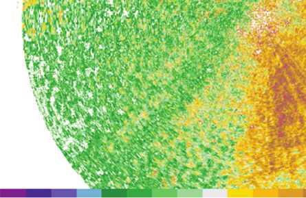
920                                      MONTHLY WEATHER REVIEW                                               VOLUME 137

                                                      FIG. 4. (Continued )

a plot of the calculated CAPE and convective inhibition         Separate frontogenesis calculations were made using the
(CIN). The CAPE values were low to the west of the              virtual potential temperature and mixing ratio fields in-
dryline but rose within the moist air until reaching a          stead of potential temperature. In both cases, the results
maximum of ;1300 J kg21 for the 2220 UTC sounding.              were similar and would not have changed the conclusions
The lowest CIN value was 19 J kg21 (sounding at 2215            reached in this paper.
UTC) but was at a location 30–40 km east of the dryline.           Low-level convergence produced frontogenesis be-
The dotted line in the middle panel of Fig. 5 identifies the    low 800 mb with a maximum .8 K (100 km)21 (3 h)21
height of the LFC. The lowest level for the LFC was             near the ground (Fig. 6a). A region of frontolysis fol-
calculated to be ;615 mb for the 2215 UTC sounding.             lowed by frontogenesis further to the east exists aloft
Accordingly, the stability analysis suggests that it would      between 700–800 mb. This couplet was created by the
be difficult to initiate convection without significant lift-   tilting term owing to descent with a minimum located at
ing provided by a convergence boundary.                         the top of the mixed layer ;100 km to the east of the
  Figure 6 shows the adiabatic frontogenesis calculated         dryline (Fig. 6b). Updrafts at the leading edge of the
from the equation in two dimensions as follows:                 dryline can also be identified in Fig. 6b. The diabatic
                                                              effect on frontogenesis was qualitatively estimated by
                   d     ›u     ›y ›u ›v ›u                     analyzing the low-level flight level data collected by the
             F5              5              ,          (1)
                   dt    ›y     ›y ›y ›y ›p                     P-3 on either side of the dryline. The dry air was
                                                                warming relative to the moist air during this period.
where the term (›u/›y)(›u/›x) has been assumed to be
                                                                Accordingly, inclusion of the diabatic term would have
small and is therefore neglected. The y direction points
                                                                augmented the frontogenesis across the dryline.
to the denser, moist air (see inset in Fig. 7). The two
terms represent the frontogenetical effects of conflu-
ence and tilting, respectively. Past studies on drylines        5. Airborne dual-Doppler analysis
have calculated frontogenesis based on the moisture
                                                                a. Horizontal structure
fields rather than temperature (e.g., Anthes et al. 1982;
Buban et al. 2007). Both the frontal boundary and                 As previously noted, the segment of the dryline that
maritime air mass to the east were well defined in the          was targeted by the P-3 was located in eastern Oklahoma
present case. Accordingly, Eq. (1) was deemed appro-            and northern Texas panhandles (Figs. 2, 3, and 4). The
priate to use to determine the frontogenetic effects.           aircraft initially performed an east–west survey pattern
MARCH 2009                                   WAKIMOTO AND MURPHEY                                                                 921

          FIG. 5. (top) Calculated CAPE and CIN values for a surface based parcel for each sounding. (middle) West–east
        vertical cross section perpendicular to the dryline of virtual potential temperature (black lines, K) and mixing ratio
        values (gray lines, g kg21). The height of the LFC is shown by the thick dotted line. The maximum height of surface-
        based parcels displaced by the dryline flow is shown by the black line. Parcel paths were calculated using the Doppler
        wind synthesis discussed later in the text. (bottom) West–east cross section perpendicular to the dryline of equivalent
        potential temperature (black lines, K) and mixing ratio (gray lines, g kg21). The locations of the soundings are shown
        by the dashed lines. The seven eastern soundings are dropsondes while the three western soundings were associated
        with balloon releases. Wind vectors are plotted using the following notation: flag 5 25 m s21, barb 5 5 m s21, half
        barb 5 2.5 m s21. The heights (AGL) are plotted for the 2233 and 2247 UTC soundings. The release points of the
        soundings are shown in Figs. 3c,d and 4c,d.

before initiating a series of flight transects oriented ap-          length in order to collect kinematic data that would re-
proximately 108–1908 (Fig. 7). The northbound (south-                veal the along-frontal variability and the mean structure
bound) legs were intended to fly on the dry (moist) side             of the boundary. The aircraft collected Doppler radar
of the primary dryline. These legs were ;100 km in                   data on the boundary for ;3 h. The tracks in Fig. 7 show
922 MONTHLY WEATHER REVIEW VOLUME 137
FIG. 6. West–east vertical cross section perpendicular to the dryline. (a) Adiabatic frontogenesis [K (100 km)21
(3 h)21], Black and dashed lines are positive and negative values of frontogenesis. (b) West–east cross section of omega
(mb s21) through the dryline. Black and dashed lines are negative and positive values of omega, respectively. Omega
was calculated using the sounding wind field and assuming no variation in the along-front direction (additional
discussion is provided in the appendix). Gray lines in both figures are the virtual potential temperature field. The
locations of the soundings are shown by the dashed lines. The seven eastern soundings are dropsondes while the three
western soundings were associated with balloon releases. Wind vectors are plotted using the following notation:
flag 5 25 m s21, barb 5 5 m s21, half barb 5 2.5 m s21. The heights (AGL) are plotted for the 2233 and 2247 UTC
soundings. The release points of the soundings are shown in Figs. 3c,d and 4c,d.
that the main dryline did not move substantially during the dryline was associated with substantial variability
the period under investigation. with pockets of maximum reflectivity ;8 dBZ. Updrafts
.2 m s21 are apparent along the northern segment of
1) 2148–2203 UTC
the dryline and appear to develop near pockets of high
The first 100-km leg flown by the P-3 was used to reflectivity as shown by Christian and Wakimoto (1989)
determine the orientation of the boundary and to po- and Wilson et al. (1994). The southerly flow was not
sition the aircraft as close as possible to the dryline. The associated with an abrupt shift in wind direction across
second leg was flown between 2148 and 2203 UTC when the dryline even though the horizontal convergence was
the aircraft was flying toward the south, parallel and to strongest along the boundary (not shown).
the east of the dryline (Fig. 8a). The airborne Doppler Also apparent in Fig. 8a are maxima in vertical vor-
radar was able to detect clear air returns out to a range ticity or misocyclones. Misocyclones developing along
of 10–15 km on this day. The thin line associated with convergence boundaries have been noted by a numberMARCH 2009 WAKIMOTO AND MURPHEY 923
ciated with the misocyclones reported in the present
study are much weaker than those shown by other in-
vestigators using ground-based radars (e.g., Arnott et al.
2006). These differences are primarily owing to the
higher spatial resolution afforded by the latter platform.
The radar refractivity plot reveals two regions char-
acterized by strong moisture gradients that were also
noted in Fig. 4 (black arrows in Fig. 8b). The western
and eastern gradients are associated with the secondary
and primary drylines, respectively. As previously men-
tioned, the apparent drying revealed in the refractivity
plot near the southern part of the aircraft track is false.
Buban et al. (2007) also noted this false drying located
southeast of S-Pol as well as a dry bias in the northern
region (see Fig. 4c). Flight-level data (not shown) col-
lected at low levels did not show a decrease in mixing
ratio from 2200 to 2204 UTC while the aircraft was
flying on the eastern side of the primary dryline. As a
result, the questionable refractivity data were removed
during the editing process. The secondary dryline was
FIG. 7. Flight track for the P-3 on 22 May 2002. The inset rep- not associated with a fine line at this time, consistent
resents the rotated coordinate system that was used to create mean
vertical cross sections for the dual-Doppler analyses shown in Fig. 8.
with the radar observations shown in Fig. 4. Weckwerth
The star denotes the location of S-Pol. et al. (2005) suggest that refractivity gradients instan-
taneously reflect moisture gradients while a fine line in
radar reflectivity requires that a concentration of insects
of investigators (e.g., Carbone 1982; Mueller and Carbone accumulate within the convergence zone before they
1987; Wakimoto and Wilson 1989; Kingsmill 1995; are detected by the radar (e.g., Achtemeier 1991).
Markowski and Hannon 2006; Arnott et al. 2006; Marquis The locations of cumulus clouds were determined by
et al. 2007). One theory for the development of these carefully superimposing visible satellite images at high
circulations is horizontal shearing instability (e.g., Miles resolution onto the radar reflectivity fields at 700 and
and Howard 1964; Carbone 1983; Lee and Wilhelmson 2500 m (Figs. 8c,d). The former and latter reveal the
1997); however, Marquis et al. (2007) have cautioned relationship of the clouds with the fine line and echoes
that it can be difficult to verify this initiating mechanism aloft, respectively. The clouds are developing over the
if misocyclones exist at the beginning of the radar ob- fine line associated with the primary dryline. Clouds are
servations. Another possible theory is that the in- also developing in the triangular-shaped region between
tersection of horizontal convective rolls (HCRs) with a the two drylines (also shown in the satellite images;
convergence boundary can produce small-scale miso- Fig. 2c). The echoes aloft (Fig. 8d) are a result of echo
cyclones (e.g., Wilson et al. 1992; Atkins et al. 1995). plumes that are associated with updrafts that form within
Buban et al. (2007) have suggested that the latter the convective boundary layer (e.g., Wakimoto et al.
mechanism may have produced misocyclones on this 2004; Miao et al. 2006). Several of the cell-shaped echoes
day and speculate that strong vertical shear-induced aloft are accompanied by clouds, which is consistent with
horizontal vortex lines could be tilted up into the base of past studies (e.g., Christian and Wakimoto 1989; Knight
the misocyclone. Buban et al. (2007) also suggest that and Miller 1993, 1998; Arnott et al. 2006; Markowski
the core vortex line in a misocyclone upwells from the et al. 2006; Buban et al. 2007; Ziegler et al. 2007). It is
near-ground level. There have been examples shown possible that some of the clouds are not being detected at
in the literature when updrafts were located immedi- this time since they are smaller than the scales resolvable
ately upstream or downstream from misocyclones (e.g., in the satellite image.
Kingsmill 1995; Murphey et al. 2006). However, there The combination of the high temporal resolution of
have been other studies that have shown no general refractivity data recorded by S-Pol and the dual-Doppler
relationship suitable for all misocyclone sizes (e.g., wind synthesis provides a unique opportunity to estimate
Marquis et al. 2007). No obvious relationship between the total derivative of radar refractivity (DN/Dt). Posi-
the updrafts and the vorticity extrema can be identified tive (negative) values of DN/Dt would suggest moisten-
in Fig. 8a. The maximum vertical vorticity values asso- ing (drying) of an air parcel. Accordingly, this quantity924 MONTHLY WEATHER REVIEW VOLUME 137
MARCH 2009                                     WAKIMOTO AND MURPHEY                                                                    925

may have utility for nowcasting of convection initiation.                 2) 2245–2254 UTC
Fabry (2006) estimated the local change of N (see his
                                                                          The analysis of the flight leg flown from 2245 to 2254
Fig. 2). Large changes in this quantity, however, could
                                                                       UTC is shown in Fig. 9. The misocyclone pattern along
be attributed to the movement of the boundary and may
                                                                       the dryline has become better defined by this time (Fig.
not significantly improve a forecaster’s ability to de-
                                                                       9a). The refractivity gradient along the secondary dry-
termine when convection might initiate.
                                                                       line is more prevalent (Fig. 9b, highlighted by the
   The total derivative was calculated by determining local
                                                                       western black arrow) and a second fine line has devel-
changes of N and the advective term (V  =N). The
                                                                       oped (Fig. 9a) as was shown in the S-Pol analysis pre-
winds based on the dual-Doppler synthesis and the dis-
                                                                       sented in Fig. 4. The air mass between the two drylines is
tribution of N from S-Pol surveillance scans were used to
                                                                       approximately represented by the refractivity values
estimate the advective terms. The local tendency of N
                                                                       that are shaded green. Clouds have formed throughout
was estimated by comparing different surveillance scans
                                                                       this region between the drylines with the largest clouds
of refractivity. The elapsed time between scans was
                                                                       located above the primary dryline (Fig. 9c). Cellular
chosen to be the same as the dual-Doppler analysis pe-
                                                                       echoes at 2500 m are located above both fine lines
riod which varied between 9 and 15 min. The plot of
                                                                       (Fig. 9d). Many of these echoes are associated with
DN/Dt is shown in Fig. 8d. The dash–dot line in the
                                                                       clouds. The DN/Dt field during this time is shown in
figure denotes the limits of the analysis area. There is a
                                                                       Fig. 9d. There is good agreement between the cloud
tendency for maxima of DN/Dt to be near regions where
                                                                       locations and the DN/Dt maxima similar to the results
clouds were developing during this analysis time. Surface
                                                                       shown during the previous analysis time.
fluxes of moisture or mixing are examples of processes
that could result in extrema of DN/Dt following a near-
                                                                          3) 2321–2333 UTC
surface parcel. These moist air parcels could highlight
favorable regions for cloud development if they were                      The reflectivity structure of the primary dryline de-
collocated with regions characterized by positive vertical             veloped a distinct along-frontal pattern during the
velocities. In this regard, the close proximity of the                 2321–2333 UTC flight leg. Striking in the analyses
DN/Dt maxima to a convergence line would be consis-                    shown in Figs. 10a,c is the resemblance of the reflectivity
tent with the visual appearance of clouds.                             pattern to the precipitation core/gap structure docu-
   Fabry et al. (1997) and Weckwerth et al. (2005) have                mented along cold fronts (e.g., Hobbs and Biswas 1979;
shown that at a temperature of 188C a change in 1 N unit               James and Browning 1979). The angle between the
can be caused by either a temperature or dewpoint                      dryline and the primary axes of the echo cores was ;208.
temperature change of 18 or 0.28C, respectively. It is                    There is a strong tendency for the misocyclones to be
important to assess whether the values of DN/Dt shown                  positioned in the gap regions between the echo cores
in Fig. 8d are reflective of moistening/drying versus                  (Fig. 10a). This relationship suggests that the circula-
temperature changes. The minimum contour of DN/Dt                      tions are contributing to the observed reflectivity
plotted in Fig. 8d is 10 3 1023 s21. If it is assumed that             structure. It should be noted that past studies of cold
the time interval between consecutive dual-Doppler wind                fronts have shown that the vorticity maxima tend to be
syntheses is 10 min, then this minimum value translates to             associated with the precipitation cores (Hobbs and
a change of N of 6 units. This corresponds to either a                 Persson 1982; Wakimoto and Bosart 2000). Kawashima
temperature change of 68C or a dewpoint temperature                    (2007) has argued that the collocation of the vorticity
change of 1.28C. The analysis shown in Figs. 8a, 9a, 10a,              maxima with the precipitation cores (i.e., locations of
and 12a do not appear to support such large changes in                 maximum convergence) suggests that horizontal shear
temperature. However, it is consistent with the type of                instability is not the likely mechanism for producing the
moisture gradients that are evident in the figure.                     variability observed along cold fronts even though it has

   FIG. 8. Airborne Doppler radar analysis for 2148–2203 UTC 22 May 2002. (a) Dual-Doppler wind syntheses, vertical velocity (red lines,
m s21), and vertical vorticity (black lines, 1023 s21) superimposed onto radar reflectivity at 700 m AGL. Surface stations are plotted with
virtual potential temperature (K), mixing ratio (g kg21), and radar refractivity (N). (b) Dual-Doppler wind syntheses, vertical velocity
(red lines, m s21), and vertical vorticity (black lines, 1023 s21) superimposed onto radar refractivity at 700 m AGL. Black arrows
represent the locations of the two drylines. Surface stations are plotted with virtual potential temperature (K), mixing ratio (g kg21), and
radar refractivity (N). (c) Cloud locations based on visible satellite imagery superimposed onto radar reflectivity at 700 m AGL. Two
sounding locations are indicated on the plot. (d) Cloud locations based on visible satellite imagery superimposed onto radar reflectivity at
2500 m AGL. Positive and negative values of total change of radar refractivity are plotted as solid red and dashed red lines, respectively.
Dashed–dot line denotes the limits of the analysis. Flight track of the P-3 is shown by the dashed line.
926 MONTHLY WEATHER REVIEW VOLUME 137
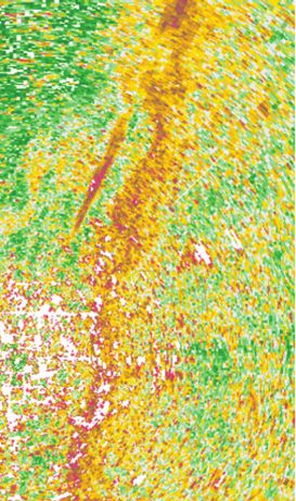
FIG. 9. Same as Fig. 8, but for 2245–2254 UTC. (b) The western and eastern black arrows denote the radar refractivity gradients
associated with the secondary and primary drylines, respectively.MARCH 2009 WAKIMOTO AND MURPHEY 927 FIG. 10. Same as Fig. 8, but for 2321–2333 UTC. (b) The black arrow denotes the location of a misocyclone that is described in the text.
928                                           MONTHLY WEATHER REVIEW                                                      VOLUME 137

                                                                        tion of moisture in a manner consistent with the previ-
                                                                        ous discussion.
                                                                           The refractivity plot continues to delineate the po-
                                                                        sitions of the two drylines (Fig. 10b) although the
                                                                        secondary dryline has retrograded since the previous
                                                                        analysis time. The secondary dryline is difficult to
                                                                        identify in the reflectivity field at low levels (Figs. 10a,c);
                                                                        however, it is prominent at higher levels (Fig. 10d). The
                                                                        opposite is true for the primary dryline (i.e., it is difficult
                                                                        to locate at 2500 m). These observations are also sug-
                                                                        gested in the results presented by Buban et al. (2007).
                                                                        This difference in echo structure in Fig. 10d suggests
                                                                        that the echo plumes/updrafts for the secondary dryline
                                                                        are stronger, which is supported by the more vigorous
                                                                        cloud development identified in the satellite image
                                                                        (Figs. 10c,d). There is a tendency for clouds to be lo-
                                                                        cated where the total derivative of N is large; however,
                                                                        the relationship is not as apparent as in the previous two
                                                                        analysis times.
                                                                          4) 2342–2357 UTC
                                                                           The primary dryline was in the early stages of propa-
                                                                        gating to the west during the last transect by ELDORA
                                                                        (2342–2357 UTC). The retrogression of the line resulted
                                                                        in a more organized updraft structure and enhanced
                                                                        cloud development (Figs. 12a,b,c). The precipitation core
                                                                        and gap structure observed earlier is less apparent in the
   FIG. 11. In situ measurements of mixing ratio (red line) at flight   radar fine line even though the misocyclones are still
level for 2321:30–2333:55 UTC superimposed on radar reflectivity        prevalent along the entire boundary.
data at 700 m AGL. Positive and negative values of vertical vor-           The secondary dryline also continued its westward
ticity are shown as solid and dashed black lines, respectively.         movement during this time. The refractivity gradient
                                                                        along the secondary dryline exhibits a wavelike pattern
been the prevailing theory that has been advanced by a                  (;15 km) after appearing more linear during the pre-
number of investigators (e.g., Parsons and Hobbs 1983).                 vious synthesis time (cf. Figs. 10b, 12b). This along-
Instead, horizontal shear instability should lead to forced             frontal variation in moisture is well matched with the
convergence between vorticity extrema as has been                       echo structure at 2500 m. This can be seen with the
shown by Lee and Wilhelmson (1997) and suggested by                     superposition of the echoes with intensity .0 dBZ
the analysis shown in Fig. 10.                                          (shaded yellow) onto the refractivity plot (Fig. 12b).
   In addition to the reflectivity and misocyclone pat-                 This is another example of the utility of radar refrac-
tern, the along-frontal variability associated with the                 tivity in locating finescale details of moisture gradients
primary dryline can be shown in a time plot of the in situ              associated with convergence boundaries and its rela-
measurement of the mixing ratio recorded at flight level                tionship with cloud development. Clouds are, in gen-
(Fig. 11). There is a several grams per kilogram varia-                 eral, positioned near regions of DN/Dt extrema (Fig.
tion of mixing ratio as the aircraft flew parallel to and               12d). It is also apparent that regions largely devoid of
west of the dryline. The dry and moist air was pre-                     clouds are located in areas with weak positive or nega-
dominantly located in the gap and echo core regions,                    tive values of DN/Dt.
respectively. There is also a tendency for the moist (dry)                 The usefulness of DN/Dt fields to facilitate nowcasts
air to be located north (south) of the misocyclone, which               of convection initiation will require further testing al-
is consistent with the results shown by Buban et al.                    though the results presented here show promise even
(2007) and also shown for a different case during IHOP                  though no thunderstorms were observed on this day.
by Murphey et al. (2006). The black arrow in Fig. 10b                   There is a suggestion that DN/Dt maxima near con-
indicates a misocyclone that is associated with a wave                  vergence lines (i.e., regions of enhanced positive verti-
pattern in the refractivity field that suggests an advec-               cal motion) could help pinpoint locations that are
MARCH 2009 WAKIMOTO AND MURPHEY 929
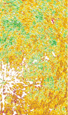
FIG. 12. Same as Fig. 8, but for 2342–2357 UTC. (d) The 0-dBZ contour for the echoes at 2500 m AGL have been superimposed onto (b)
the refractivity plot and are shaded yellow.930 MONTHLY WEATHER REVIEW VOLUME 137
favorable for storms to develop. Forecasters should be 22 May 2002 2148:35 - 2203:14 UTC
able to derive this variable even in the absence of dual- dBZ
Doppler wind syntheses. Horizontal wind fields at low ζ
x 10-3 s-1
levels used to estimate advection can be approximated -2
2
by tracking the movement of clear air echoes (e.g., 0
Tuttle and Foote 1990); tracking echoes and adding a 2 0
1
0
constraint using the radial velocity momentum equation km
0
0.5
AGL
(e.g., Laroche and Zawadzki 1995); or by combining
0
10 m / s
meteorological observations, and a numerical boundary 4 km a 2148:35 - 2203:14 UTC
layer model and its adjoint (Sun and Crook 2001). In 10
this regard, the DN/Dt analysis is seen to be superior to V’
W
-0.5
combining the low-level convergence field with an N
6
8
2
analysis. The latter technique requires the identification 4
1.0
of small pockets of convergence (i.e., updrafts) that can
only be accurately resolved using a dual-Doppler wind
1 .5
1
km
0.5s
m/
synthesis. These detailed wind syntheses would often be 2
AGL /s
0.5
m 0 -2
unavailable to a forecaster.
4 km
22 May 2002 2342:00 - 2357:01 UTC
b. Vertical structure
dBZ
The long legs flown by the P-3 provided an opportu- ζ
x 10-3 s-1
nity to properly assess the along-frontal variability of 2
-2
the dryline. The voluminous amount of wind data col- 0 0
lected during these transects were also used to construct 0
2
1
0.5 0
mean vertical cross sections oriented perpendicular to km
0
AGL
the primary dryline. The horizontal grid spacing of the 10 m / s
Doppler wind syntheses was 600 m, as described in the 4 km
b 2342:00 - 2357:01 UTC
appendix. Although the number varied slightly for each 8
V’ 4
analysis time, ;105 cross sections were averaged for W
each flight leg (Fig. 13). The mean structures shown in 6
2
-1.0
the figure should be largely devoid of the variability 4
1.0
3.0
2.0
2
0
along the dryline. 0
m/ s
0.5
The mean vertical cross section for the analysis shown 1 -2
1.0
km
in Fig. 8a is presented in Fig. 13a. The thin line echo can AGL -4
m/s
be seen in the top panel with maximum reflectivities
greater than 4 dBZ. Peak updrafts over the dryline were 4 km
greater than 1.5 m s21. There is a head structure with FIG. 13. Mean vertical cross sections perpendicular to the dry-
weak downdrafts to the east of the dryline. There is a line for (a) 2148:35–2203:14 and (b) 2342:00–2357:01 UTC 22 May
slight veering of winds with increasing height through 2002. (top) Radar reflectivity (dBZ) is plotted as gray lines with
values greater than 2-dBZ shaded gray. Positive values of vertical
the maritime air mass. Mean cyclonic vorticity greater
vorticity (1023 s21) are plotted as thin black lines. Vertical ve-
than 0.5 3 1023 s21 associated with the misocyclones locities and component of horizontal flow in the plane of the cross
extends up to 1 km. Shallow, easterly flow can be seen in section are plotted as black arrows. (bottom) Positive and negative
the component of horizontal flow perpendicular to the values of vertical velocity (m s21) are plotted as black and dashed
dryline (y9) east of the dryline (Fig. 13a, bottom panel). lines, respectively. Component of horizontal flow (m s21) per-
pendicular to the boundary is plotted. Positive (easterly) and
Enhanced return flow can be seen above the maritime
negative (westerly) flow are shown by the gray and dashed gray
air mass. A rotor circulation generated by the solenoi- lines, respectively. The rotated coordinate system is shown in the
dal circulation is located east of the fine line. Miao and inset in Fig. 7.
Geerts (2007) state that no circulation existed across the
dryline during this time. This inconsistency is likely the
result of the analysis of a single cross section in their study The structure during the period when the dryline
versus the average of numerous cross sections presented was beginning to move westward is shown in Fig. 13b.
in this article. In addition, a rotor circulation is evident The easterly flow within the maritime air mass has in-
in the analysis presented by Weiss et al. (2006). creased in magnitude and depth. The peak updraftsMARCH 2009 WAKIMOTO AND MURPHEY 931
have increased (.3 m s21) and shifted to the western strongest shear (largest negative values of horizontal
edge of the fine line. The rotor circulation is better de- vorticity) is located ;100 km to the east of the dryline.
fined and deeper at this time, consistent with the results The spacing of the sounding data is insufficient to fully
presented by Miao and Geerts (2007). Mean surface- resolve the rotor circulation (the position of the center
based trajectories were calculated using the dual-Dop- of the rotor is shown by the cross in Fig. 14).
pler wind syntheses from 2321 to 2333 UTC and 2342 to The horizontal vorticity equation can be simplified as
2357 UTC (and a backward time difference scheme) by follows:
releasing air parcels at the lowest grid point in a line
perpendicular to the dryline. The maximum height that Dj ›B
5 , (2)
surface-based parcels would attain (indicated by the Dt ›y
black line in the middle panel in Fig. 5) is far below the
where B is the buoyancy, the flow is assumed frictionless,
height of the LFC suggesting that convection initiation
and there are no along-frontal variations. It is also as-
would be unlikely on this day. In contrast, Buban et al.
sumed that tilting of vorticity is small (Sipprell and
(2007) suggest parcel trajectories reaching a higher
Geerts 2006; Buban et al. 2007). The solenoidal term is
level. They showed that the air parcels from both west
shown in Fig. 14b and reveals that most of the air mass
and east of the dryline were associated with insufficient
east of the dryline and beneath the capping inversion
CAPE to initiate convection even if they attained
was generating negative horizontal vorticity with a
heights between 2.5 and 3.5 km. The present study used
minimum ,22 3 1026 s22. Buban et al. (2007) pre-
the wind field averaged along the length of the dryline in
sented values that are approximately 5 times larger
order to examine the mean lift along the boundary. This
concentrated within a narrow 1-km zone using the
would underestimate the maximum heights of individ-
higher-resolution data contained in their Lagrangian
ual parcels that are captured in the study by Buban et al.
analysis. Their background values to the east of the
(2007). In addition, the dual-Doppler syntheses do not
dryline were ;1 3 1026 s22, consistent with the meso-
include the three-dimensional winds from the surface to
scale analysis presented in this study. The solenoidal
the top of the boundary layer, which would preclude
term is positive aloft and to the east of the dryline owing
deep trajectories. Surface-based CAPE estimates may
to the reversal of the horizontal temperature gradient to
also underestimate the maximum attainable parcel al-
the rear of the ‘‘head’’ of the maritime air mass. The
titude versus a layer-averaged value at low levels.
advective terms were calculated (not shown) in order to
The resemblance of a retrograding dryline to a den-
assess the tendency of j (Fig. 14b). The tendency is
sity current has been documented before (e.g., Parsons
negative at low levels (,1.5 km) but there are several
et al. 1991; Ziegler et al. 1995; Murphey et al. 2006;
regions where minimum values are ,22 3 1026 s22.
Sipprell and Geerts 2006). The solenoidal-generated
One of the areas located near the 2150 UTC sounding at
circulation is believed to be the primary mechanism for
;800 mb is nearly collocated with the rotor circulation
the generation of horizontal vorticity within the head of
resolved by the dual-Doppler wind synthesis. Accord-
the density current (e.g., Sun and Ogura 1979; Ziegler
ingly, the coarse resolution sounding analysis illustrates
et al. 1995; Sipprell and Geerts 2006; Miao and Geerts
the importance of the solenoidal generation of hori-
2007). Sipprell and Geerts (2006) estimated the vortic-
zontal vorticity and updrafts at the leading edge of the
ity generation owing to baroclinic effects using in situ
maritime air mass similar to past studies. Frontogenesis
data collected by an aircraft. Buban et al. (2007) used a
would also promote positive vertical motion in the
Lagrangian analysis of thermodynamic variables based
warm sector; however, this was insufficient to initiate
on high resolution dual-Doppler wind syntheses and
convection.
in situ data collected by a mobile mesonet, aircraft, and
sounding data to document the solenoidal genera-
6. Summary and conclusions
tion of the horizontal vorticity. In the present case, the
changes in horizontal vorticity (j) and the solenoi- A detailed analysis of a dryline that formed on 22
dal effects in the vertical plane perpendicular to the May 2002 during IHOP was presented. An airborne
primary dryline were estimated using the thermody- Doppler and a ground-based multiparameter radar were
namic and wind data from the soundings presented in the primary platforms used in this study. The former
Fig. 5. flew long legs (;100 km) at low levels that were parallel
A band of negative vorticity ,28 3 1023 s21 is lo- to the boundary in order to collect data that would
cated near the capping inversion (Fig. 14a) and is in resolve the along-frontal variability of the dryline. In
response to the strong vertical wind shear between the addition, averaging of numerous cross sections of the
maritime air mass and the dry, westerly flow aloft. The Doppler wind syntheses revealed the mean vertical932 MONTHLY WEATHER REVIEW VOLUME 137
2247 2235 2150 2215 2217 2220 2224 2227 2230 2233 UTC
600
mb θv
318
ELDORA ξ max
X ξ
< -8 x 10⁻³ s-1
-4
x10-3s-1
3
317
-4 3
700 3 316
31 0
2 312 315
-4
311
0 2
800
1
X -12
km -16
AGL
-8 1
km
900 -4 AGL
20 cm/s
30
30
30 K
20 m/s
5
1
2
a 100 km
2247 2235 2150 2215 2217 2220 2224 2227 2230 2233 UTC
600
mb ∂ B/ ∂ y ∂ξ /∂t
x10-6s-2 x10⁻⁶s-2
3
0.5
3
700
2
.5 -2
-0 0.5
2 0
2
0
-1
800
1
X
-2 -1.5
km
AGL
-2 1
-2 km
900 -2 AGL
20 cm/s
20 m/s
b 100 km
FIG. 14. West–east vertical cross section perpendicular to the dryline. (a) Horizontal vorticity (j) parallel to the
dryline (black lines, 1023 s21) and virtual potential temperature (gray lines, K). (b) Tendency of the horizontal
vorticity (black lines, 1026 s22) and solenoidal effects generated by the horizontal gradient of buoyancy (gray lines,
1026 s22). Black arrows on both plots represent the total vertical velocity and the component of horizontal flow in the
plane of the cross section. The black cross represents the location of the rotor circulation shown in Fig. 13. The locations
of the soundings are shown by the dashed lines. The seven eastern soundings are dropsondes while the three western
soundings were associated with balloon releases. The heights (AGL) are plotted for the 2233 and 2247 UTC soundings.
The release points of the soundings are shown in Figs. 3c,d and 4c,d.
structure of the dryline. The S-Pol radar provided con- from the boundary layer based on the mean dual-
tinuous surveillance scans of the dryline and was equip- Doppler wind syntheses. Another study of this case
ped with the capability to record refractivity. Variations showed that air parcels were associated with insufficient
of radar refractivity are primarily caused by changes in CAPE to initiate convection. The formation of a sec-
water vapor under typical summertime conditions. ondary dryline located to the west of the primary dry-
The 22 May dryline was classified as a null case since line was also documented on this day. The secondary
no convection initiated along the boundary on this day. dryline was apparent in the reflectivity data as a fine line
The absence of deep convection is supported by the and in the refractivity analysis as a distinct moisture
analysis of a series of soundings that revealed the height discontinuity.
of the LFC at ;620 mb. This level was significantly The kinematic structure of the primary dryline re-
greater than the maximum height for air parcels lifted vealed substantial along-frontal variability. Indeed, theMARCH 2009 WAKIMOTO AND MURPHEY 933
reflectivity pattern during one of the analysis times was often mask the cumulus cloud field at lower levels lim-
remarkably similar to the precipitation core/gap struc- iting the utility of forecasting convection initiation using
ture documented along cold fronts. Circulations asso- satellite imagery alone (e.g., Weckwerth et al. 2005). In
ciated with misocyclones were positioned in the gap addition, high values of DN/Dt near a convergence line
regions and contributed to the observed echo pattern. might precede the appearance of clouds on a visible
The misocyclones were advecting moist (dry) air, as satellite image. Unfortunately, the coarse temporal res-
shown in the refractivity analysis and the in situ data olution of the dual-Doppler wind syntheses did not allow
collected at flight level, in the regions north (south) of for an accurate assessment of the latter.
the circulations. Similar distortions of the moisture fields The forecaster also requires knowledge of whether
by misocyclones have been shown in past studies. lift is sufficient to carry parcels to the LFC (it was in-
A pronounced maritime air mass with a strong cap- sufficient in the present case), the existence of midlevel
ping inversion was identified in the vertical cross section entrainment that may inhibit convective growth, and
through the dryline. The dryline was undergoing front- whether the vertical circulation associated with deep
ogenesis of the potential temperature field. The hori- convection is surface-based (e.g., Banacos and Schultz
zontal circulation within the head at the leading edge of 2005). The main constraining factor in deriving DN/Dt
the maritime air mass was shown to be primarily driven is the short range over which refractivity data can be
by solenoidal effects. The largest values of horizontal collected (40–60 km). In spite of this limitation, the
vorticity were located ;100 km to the east of the dryline observations presented in this paper are quite promising
and were in response to the strong vertical shear across and suggest that future studies should continue to focus
the inversion. on the utility of this variable for nowcasting of deep,
The positions of cumulus clouds using high-resolution moist convection.
satellite images were superimposed onto the S-Pol re-
flectivity data. The clouds were forming over the pri- Acknowledgments. Research results presented in this
mary and secondary drylines and within the air mass article were partially supported by the National Science
between the two boundaries. Many of the clouds were Foundation under Grant ATM-021048. The National
collocated with clear air echoes aloft (2500 m). These Center for Atmospheric Research is sponsored by the
echoes were associated with updraft plumes that formed National Science Foundation. Any opinions, findings,
within the convective boundary layer and were often and conclusions or recommendations expressed in this
located at the leading edge of strong gradients of re- publication are those of the authors and do not neces-
fractivity. sarily reflect the views of the National Science Foun-
Past studies of radar refractivity have focused on its dation. Comments from Jim Wilson and Rita Roberts
ability to accurately assess the low-level moisture fields; substantially improved an earlier version of this manu-
however, its use in forecasting has been restricted to script. Constructive criticism provided by anonymous
qualitative interpretations. This study introduced the reviewers is also acknowledged.
total derivative of radar refractivity (DN/Dt) in order
to quantitatively assess its ability to improve the pre-
diction of the initiation of convection. There was a gen- APPENDIX
eral tendency for maxima of DN/Dt to be near regions
where cumulus clouds were developing along a fine line.
Analysis Methodology
The collocation of these maxima near a convergence
line where favorable vertical velocities exist may help The radar data were edited and the aircraft motion
identify preferred regions for convection initiation. Al- was removed from the velocity fields using the SOLO II
though dual-Doppler wind syntheses were used to cal- software package (Oye et al. 1995). The data were then
culate DN/Dt, current techniques are available to esti- corrected for navigation errors using a technique de-
mate the horizontal wind field in the boundary layer veloped by Testud et al. (1995). The along-track and
using single-Doppler radar data. Accordingly, it should sweep-angle resolution for ELDORA during IHOP was
be possible for forecasters to make good estimates of this ;600 m and 1.58, respectively, based on the information
derivative. presented in Table 1. The sweep angle resolution led to
While the locations of the cumulus cloud field can be an effective sampling in the vertical of ;300 m for the
obtained currently from high-resolution satellite im- maximum distances from the radar used in the present
ages, an analysis of DN/Dt provides important infor- study.
mation on the evolving water vapor field following an The radar data were interpolated onto a grid with a
air parcel. It should also be noted that cirrus clouds can horizontal and vertical grid spacing of 600 and 300 m,You can also read