Anwendung künstlicher Neuronaler Netze in der Optimierung - Mike Steglich Künstliche Intelligenz - verständlich
←
→
Page content transcription
If your browser does not render page correctly, please read the page content below

Anwendung künstlicher Neuronaler Netze in der Op8mierung

 Anwendung künstlicher Neuronaler Netze in der Optimierung

 Mike Steglich
 Technische Hochschule Wildau

 Künstliche Intelligenz -> verständlich

 06. Juli 2020

Anwendung künstlicher Neuronaler Netze in der Op8mierung

 Zwei gegensätzliche Welten?

 Künstliche Neuronale Netze (KNN) Optimierung

 = → ! ( !)
 . . .
 ≥

 ?
 ! = 0; ∈ 1,2, … ,
 ≤
 ≥0

 Künstliche Neuronale Netze sind parallel verbundene Bestimmung des Lösungselementes mit dem
 Netzwerke aus einfachen Elementen in hierarchischer besten Zielfunktionswert aus einer Menge
 Anordnung, die mit der Welt in der selben Art wie zulässiger Lösungselemente.
 biologische Nervensysteme interagieren sollen.
 (Kohonen 1982)

 Abbildung eines Inputvektors auf einen Output-
 vektor

Mike Steglich – KI verständlich – 06. Juli 2020 2
Anwendung künstlicher Neuronaler Netze in der Op8mierung

 Künstliches Neuronales Netz (KNN)

 o KNN sind als gerichteten Graphen darstellbar, die sich durch eine Menge von Knoten (Neuronen) und
 eine Menge von bewerteten Kanten beschreiben lassen.
 o Die über die gewichteten Kanten übertragenen Argumente werden in den Knoten (als eigentliche
 Berechnungseinheiten eines künstlichen neuronalen Netzes) über bestimmte Berechnungsvorschriften zu
 einen Outputwert moduliert. (Zell 1997)

 w[1]11
 e1 h1 w[2]11
 [1]
 w 21
 1
 [1]
 w[2]21
 ( )
 w 31
 o1 h= sW [1]
 ×e 0.8
 w[1]12 w[2]12 0.6
 e2 w[1]22
 h2 w[2]22 0.4

 ( )
 [1]
 w 0.2
 32
 o = s W [2] × h
 w[1]13 w[2]13 o2
 w[2]23 -10 -5 5 10

 w[1]23
 e3 h3
 w[1]33

 (Steglich 2001, S. 215)

Mike Steglich – KI verständlich – 06. Juli 2020 3
Anwendung künstlicher Neuronaler Netze in der Op8mierung

 Künstliches Neuronales Netz (KNN)

 o Die Aufgabe eines KNN besteht darin, die Abbildung vom Inputvektor auf den Outputvektor zu
 erlernen und zu repräsenMeren.

 1 1
 2 2

 o Ein KNN arbeitet in zwei Modi:
 § einer Lernphase und
 § einer Ausführungsphase (Recallphase).

 o In der Lernphase werden die Kantengewichte zur Abbildung : ! → " in der Lernphase durch einen
 Lernalgorithmus festgelegt.
 § Überwachtes Lernen erfolgt anhand von Beispielen mit Eingabe- und zugehörigen Ausgabewerten.
 § Unüberwachtes Lernen erfolgt anhand von Beispielen einzig mit Eingabewerten.

 (Aggarwal 2018, S. 4ff, Rojas 1996, S. 29)

Mike Steglich – KI verständlich – 06. Juli 2020 4
Anwendung künstlicher Neuronaler Netze in der Op8mierung

 Zwei miteinander verbundene Welten

 KNN als Pre- bzw. Post-
 OpMmierung als
 Processing der Daten für
 Bestandteil des KNN-
 eine OpMmierungsan-
 Lernalgorithmus
 wendung

 KNN als Bestandteil eines
 Optimierungsalgorithmus

Mike Steglich – KI verständlich – 06. Juli 2020 5
Anwendung künstlicher Neuronaler Netze in der Op8mierung

 Zwei miteinander verbundene Welten

 o KNN als Pre- bzw. Post-Processing der Daten für eine Optimierungsanwendung

 = → ! ( !)
 . . .
 ≥
 ! = 0 ; ∈ 1,2, … ,
 ≤
 ≥0

 Data pre-processing Data post-processing
 zur Bes2mmung von zur Analyse der
 Problemdaten Lösung

Mike Steglich – KI verständlich – 06. Juli 2020 6
Anwendung künstlicher Neuronaler Netze in der Op8mierung

 Zwei miteinander verbundene Welten

 o Optimierung als Bestandteil des KNN-Lernalgorithmus

 (Schaaf 2020)

Mike Steglich – KI verständlich – 06. Juli 2020 7
Anwendung künstlicher Neuronaler Netze in der Op8mierung

 Zwei miteinander verbundene Welten

 o KNN als Bestanteil eines Optimierungsalgorithmus (i.d.R. Heuristik)

 § KNN als eigenständiger Optimierungsalgorithmus
 § KNN als Bestandteil eines Optimierungsalgorithmus

Mike Steglich – KI verständlich – 06. Juli 2020 8
Anwendung künstlicher Neuronaler Netze in der Op8mierung
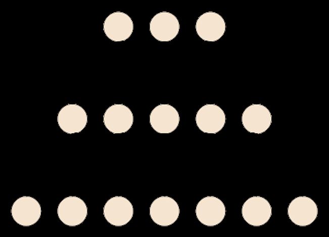
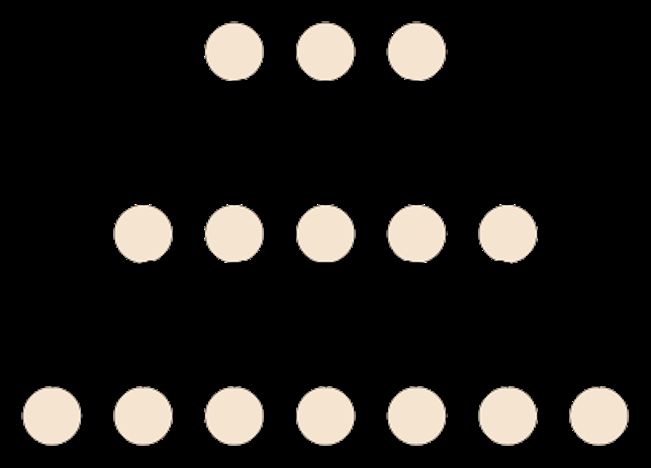
Self-organising maps (SOM)
o A SOM is able to find a topographical projecMon ∶ → , where describes input paWerns of
aWributes and a usually one- or two-dimensional representaMon of the input paWerns (Kohonen 1982).
o A SOM can be described as a feed-forward network consisMng of two layers of units. The input units are
completely connected with the output units in the second layer. The weights on the edges between the
8 formulated as a Matrix = {
input and output units can be Mike Steglic
#$ ∈ ℝ | ∈ {1,2, … , }, ∈ {1,2, … , }}
(Kohonen 1982).
o1 o2 o3
w11 w43
i1 i2 i3 i4
Fig. 1 Example of a SOM with an one-dimensional array of output units
(Steglich 2019)
Mike Steglich – KI verständlich – 06. Juli 2020 9alternating location-allocation
Fig. 1 Example
unit have to be updated heuristic:
of a SOM withSince the projection
an one-dimensional
in order to improve the matching. between
array of outputthe input unitspatterns and the ac-
n heuristic:
found in the first Since steptheisprojection
used in between a ca- the tivity input of the output
patterns and the unitsac- have to be topographically cor-
LA Anwendung künstlicher Neuronaler Netze in der Op8mierung
d inheuristic
a ca- to find and improve
tivity
Theofoutputthe output a solution
units unitsarehave usually torect, the
beorganised weights of thecor-
topographically neighbours of the winner unit also
as a one- or two-dimensional array,
MP. The allocationrect,
a solution of thethedestinations
weights to the
of the have oftothebewinnerupdated. Kohonen
also proposed the Gaussian neigh-
where the units are neighbours
laterally connected. unit
based
ions toon thea GAP have whichtoisbesolvedupdated. by Kohonen
using proposed bourhood the to function as
Gaussian neigh- shown in expression (8) for a one-
Self-organising maps
The (SOM)
projection f : ⇥ ! ⌦ has be found during
cing
d by technique
using and variablefunction
bourhood relaxing-fixing as shown in dimensional
expression array
(8) for ofaoutput
one- units,the whereso-called
s defines learning
the width
The locations phase, which means, that the following steps have to be carried on T = e·N
xing-fixing o Theare modified :by
dimensional
projection
times,
where
determining
array
→ ofhas
estepsoutput
is the to units,
be found of the
where kernel
during
number of so-called epochs.s defines
the (Kohonen,
the width
so-called 2001,
learning p. 111).
phase, which means that the
setermining
for each allocation cluster.
of the kernel Both
(Kohonen, are
2001,out p. 111). !
following stepsGiven have antoinputbe carried vector ✓lseveral
2 ⇥ =times {✓m |m (Kohonen,
2 {1, 2001,
2, .h) .p..2106) . l 2 {1, 2, . . . , L},
, I}};
long as
h steps are improvements for the CPMP occur ! layer (n
ution for a 1. Initialisation:
continuous, only one
capaci- Initialise
unit of the all
Afterweights
output 2 by
finding thed (n,
assigning h) =be
can
winning exp
randomactivated
output values.
unit, 2according
; n 2 {1, 2,the
tothis O}.
. . . ,winner- (8)
um number
PMP occur of steps is not reached. (n h) 2sthe weights of
y solving aoptimisation
GAP. d (n,
takes-all h) = exp
output function
unit have be; ninput
(8). 2 {1, 2,
This is in. the , O}.
. . orderoutput(8)unit ⌘the 2 {1, 2, . . . , O} with
hbourhood
d. 2. Propagation: heuristic:Choose In the last2s 2 toan
randomly updated pattern % ∈to improve = { # | ∈matching. {1,2, … , }}; ∈
stlocation-allocation
solution
In the last found so heuristic:
the
far minimum
is improved Since
squared
by us-
{1,2, … , } and determine the winner unit the projection
Euclidean To between
distance
update a the
between
weight inputw mn patterns
the
between input andan the
vector
input ac-unit
✓l and its an
m and
he
lved first step is used
neighbourhood
by us- Toinupdate
weight
optimisationa ca-vector wtivity
aheuristic.
weight n . Inof the output unit
wmn between an input unitsn,unit have
them toandbeantopographically
difference (qm wmn ) iscor- multiplied by the
2
to find and
subregion,
uristic. In improve
surrounding a solution
output a selected
unit rect, the (q
median,
n, the difference weights of) the
⌘ = neighbourhood
arg
wmn ismin neighbours
multiplied k✓lbydof
value wthe
(n,
the nh)k winner unit also factor
and a learning-rate (8)a as
m n2{1,2,... ,O}
ation
edf the of the destinations
solution
median, found for tothis
neighbourhood thesubregion
value have (n,toh)
d im- beandupdated.
shown Kohonen
in the learning
a learning-rate proposed
factor aruleasthe
(9) Gaussian
(Kohonen,neigh- 2001, p. 111).
AP
bjective
region which
im- is solved
function value
shown byofAfter
using
thethe
in entire
finding
learning bourhood
problem,the (9) function
winning
rulewinner (Kohonen, output as2001,
shown
unit, p. in theexpression
111). weights of (8)thisfor unit
a one-have to be
e problem,
and variable 3. Updating
relaxing-fixing weights for the
dimensional and
array its neighbourhood
of matching.
output Dwunits, where :
a · d (n, s h) · (qm thewwidth
defines
tial
re solution updates the entire in
updated solution.
order This
to improve the mn = Since the projection )
mnbetween the
are
sution. modified
repeated Thisuntilby all determining
medians
inputs
Hybrid areDw
patterns mn =of
optimised
heuristic a
and
forthe or
· dthekernel
the
(n, h) (Kohonen,
activity
· (q
capacitated m of the
mn )2001,
wp-median ;output p.
m 2problem{1,111).
2, . . . ,have
units I}, n 2 to{1,be2,topographically
. . . , O} (9)
9
ocation
number
ptimised or cluster.
of steps Bothwith steps
no
correct, are
improvements
the weights is of the neighbours
; m 2 {1, 2, . . . , I}, n 2 {1, 2, . . . , O} 2 of !the winner
(9) unit also have to be
ovements
vements is for the CPMPupdated.occur Kohonen proposed Both
the parameters
(n
Gaussian h) a and
neighbourhood s are usually function decreasedas shownin each
2. Propagation: Choose d (n, h) = exp
randomly
step of the
an input ;pattern
learning n
phase2 {1, 2,✓.l .2
to ensure . , O}.
⇥
faster (8)
and determine
changes
the
of the
steps is not reached.in Both parameters
expression (9) a and
for a s are usually
one-dimensional 2s
decreased 2
array inof each
output units, where defines
winner unit ⌘ using expression (8). t
timisation heuristic:
GAP-based heuristic stepInto the
of lastlearning
solve
the a of
continuous, phase
kerneltoin ensureweights faster in achanges
broader neighbourhood at the beginning of the
the3.widthUpdating theweights: learning
Update all step
weights t [32]. byofusing the the learning rule (10) and
und so far
median
ontinuous, is improved
problem weights byinus-a broader To update
neighbourhood alearning
weight
at the process
w beginning
mn and
between to
of
! with step 2. anrefine
the input it at
unitthe m end
and ofanthe process.
4.
ood optimisation heuristic. Stop, if a stopping
decrease rule
In
↵ and is satisfied
. or else
Afterwards, continue for all w patterns ✓l 2 ⇥ theby corresponding out-
scribes the generation learning process
of4.a solution
Stop, a output
and
if for tocon-
a(n,
stopping ⌘)
unitit
refine
=
n,atthe
rule
exp
the
is difference
end
(n of ⌘)
satisfied the2or
(qprocess.
melse
; n 2
mn ) is multiplied
continue
{1, 2, . . .with
, O}. stepthe 2. (9)
urrounding a selected median, for allneighbourhood
Afterwards, patterns ✓ 2 puts
⇥ valuehave
the d to be
h)
corresponding
(n, 2 determined
and a by
learning-rate
out- applyingfactor thea winner-takes-all
as
tatedfor ap-median problem using a SOM and a l 2
nn found con- t
for this subregion im- shown in the function:
learning rule (9)the (Kohonen, 2001,
SOM and
puts have Afterwards,
to be determined for
o a Afterwards, for all patterns % ∈ the corresponding all
by patterns
applying ✓
thel 2 ⇥
winner-takes-all
outputscorresponding
have to p.be111).
outputs
determined havebyto be
applying the
ion value ofwinner-takes-all
the entire problem,
determined
function: function:
To update by applying the
a weight wmn between anwinput winner-takes-all function:
unit m and
pdates the entire solution. This Dwmn = a · d (n, h) l =· (qargm wmin mn ) k✓an l woutput
nk
2 unit n,
maps the di↵erence (✓!m = w mn ) ismin multiplied k✓2 l by wnthe neighbourhood
k2 ; ln2{1,2,...
2 {1, 2, ,O}
. . . , L}.value (n,(11) ⌘)
il all medians are optimised or wl = argl arg minn2{1,2,...
; m k✓2 l {1, w 2,
n k. . . , I}, n 2 {1, 2, . . . , O} (9)
and a learning-raten2{1,2,... factor,O} ↵t as shown ,O} in; l the
2 {1, learning
2, . . . , L}. rule (10). (10)
rticular
teps withtypeno of an artificial is
improvements neural network
uced by Kohonen (1982).wmn
al network The=main
There ;↵lare
2 charac-
{1, 2, . . . parameters
Both
obviously , L}.some a) and
similarities s {1,arebetween .(10)
usually decreased {1,in
a Self-Organising 2, each Map and
t · (n, ⌘) · (✓m SOM-based wmn 2
; mapproach 2, . . solve
to , I}, na 2continuous, . . . uncapacitated
, O} (10)
OMain is the capability toafind
charac- a topographical
continuous, step of the learning
uncapacitated phase toproblem
p-median ensure faster [11, 45]. changes
Therefore,of the Lozano et
SOM-based approach to solve a p-median problem
continuous, uncapacitated
⇥euristic
!Mike
pographical where
to solve
⌦, Steglich –⇥ describes
KIaverständlich
continuous,
al.,
Both –L06.
Hsieh input
Juliand
2020
parameters weights
patterns
Tien ↵and in a broader
t and Arast et areneighbourhood
al.usually
proposed at the beginning
several
decreased in eachofstep
SOM-based theapproaches
t of the 10Anwendung künstlicher Neuronaler Netze in der Op8mierung Self-organising maps (SOM) (Eigenes Experiment) Mike Steglich – KI verständlich – 06. Juli 2020 11
Anwendung künstlicher Neuronaler Netze in der Op8mierung

 Lösung des symmetrischen Rundreiseproblems miHels selbstorganisierter Karten

 o Mit diesem Problem ist die kürzeste geschlossene Reiseroute über eine Anzahl von Orten zu finden. Die
 Distanzen zwischen den Orten sind bekannt. Jeder Ort muss mindestens bzw. möglichst genau einmal
 aufgesucht werden. Anschließend wird zum Ausgangsort zurückgekehrt (Steglich et al. 2016, S. 278 f).

 Parameter:
 åc ij × xij ® min!
 Menge der Knoten
 [i , j ]ÎA
 s.t . Menge der Kanten
 ( ) Menge der mit dem Knoten inzidenten Kanten
 åd xij = 2 ;i Î N
 [i , j ]Î ( i ) ( ) Menge der mit den in der Menge enthaltenen Knoten
 verbundenen Kanten
 å xij £ S - 1 ;S Ì N , S ³ 2
 [i , j ]Îd ( S ) Distanz der Kante , ∈
 xij Î{0,1} ;[ i , j ] Î A Variablen:
 Kantenindikatorvariable , ∈
 (Steglich et al. 2016, S. 281 f., Chen et al. 2010, S. 146 ff., Ghiani et al. 2013, S. 368 ff.]
Mike Steglich – KI verständlich – 06. Juli 2020 12
Anwendung künstlicher Neuronaler Netze in der Op8mierung Lösung des symmetrischen Rundreiseproblems mittels selbstorganisierter Karten o Die Anzahl möglicher Touren beträgt bei einem symmetrischen Rundreiseproblem − 1 !/2. &! o Bei 10 Knoten exisMeren ( = 181.440 unterschiedliche Touren. ()! o Bei 26 Knoten exisMeren ( = 7,76 I 10(* Varianten, die bei einer Bearbeitungszeit von einer Millisekunde pro Variante 7,76 I 10(* Millisekunden bei einer vollständigen EnumeraMon benöMgen würden. o Zum Vergleich: Das geschätzte Alter des Universums beträgt 13,7 Milliarden Jahre ≈ 4,32 I 10(* Millisekunden (Vgl. Sperkel et al. (2003)). (Vgl. Steglich et al. 2016, S. 285.) Mike Steglich – KI verständlich – 06. Juli 2020 13
Anwendung künstlicher Neuronaler Netze in der Op8mierung

 Lösung des symmetrischen Rundreiseproblems miHels selbstorganisierter Karten

 o Bei vorliegenden Städten besteht die Ausgabeschicht aus einer ein-dimensionale Karte mit insgesamt
 ringförmig angeordneten Knoten.
 o Als Eingaben werden die Koordinaten der Städte verwendet. Durch den Lernprozess spezialisiert sich
 jeder Knoten der Ausgabeschicht auf eine Stadt. Es entsteht eine eine Rundreise über alle Städte.

 (Eigenes Experiment unter Verwendung der Software Sikone / Uni Halle)

Mike Steglich – KI verständlich – 06. Juli 2020 14
Anwendung künstlicher Neuronaler Netze in der Op8mierung

 Lösung des konJnuierlichen, unkapaziJerten p-Median-Problems miHels SOM

 o Eine Anzahl von Bedarfsorten ist auf
 einer ebenen Fläche oder auf einer
 Kugeloberfläche verteilt. Es werden
 Standorte (Angebotsorte) zur
 Bedienung der Bedarfskonten gesucht.
 o Die einzelnen Punkte auf einer ebenen
 Fläche oder auf einer Kugeloberfläche
 stellen die PosiMonen der potenMellen
 Standorte dar.
 o Es sind die PosiMonen der Standorte
 sowie die opMmale Zuordnung der
 Bedarfsknoten zu den Angebotsorten zu
 besMmmen, wobei die Summe der
 Distanzen zu minimieren ist.

 (Steglich et al. 2016, S. 402 ff., Winkels 2012, S. 416 f.)
Mike Steglich – KI verständlich – 06. Juli 2020 15
Anwendung künstlicher Neuronaler Netze in der Op8mierung

 Lösung des konJnuierlichen, unkapaziJerten p-Median-Problems miHels SOM

 Indexmengen:
 E E !$ ⋅ ! , ! , $ , $ → min!
 !∈# $∈%
 ! – Menge der Standorte, |!| = $
 . . . % – Menge der Bedarfsorte
 Indizes:
 E !$ = 1 ; ∈
 & – Index der Standorte, & ∈ !
 !∈#
 !$ ∈ 0,1 ; ∈ , ∈ ( – Index der Bedarfsorte, ( ∈ %
 Parameter:
 $ – maximale Anzahl von Standor-
 ten
 (*! , ,! ) – Koordinaten des Bedarfsortes
 (∈%
 Variablen:
 (." , /" ) – Koordinaten des
 Standorts & ∈ !
 *"! – Zuordnungsvariable des Bedarfsortes (
 zum Standort &
 1(∙) – Distanzfunktion zwischen einem Stand-
 ort und einem Bedarfsort

 (Steglich et al. 2016, S. 402 ff., Winkels 2012, S. 416 f.)

Mike Steglich – KI verständlich – 06. Juli 2020 16
Anwendung künstlicher Neuronaler Netze in der Op8mierung

 Lösung des konJnuierlichen, unkapaziJerten p-Median-Problems miHels SOM

 One input unit per There are p
 coordinate; one output units,
 paGern represents which
 Map with the coordinates of represent areas
 the a des2na2on of the map
 locations
 aJer the
 of the
 learning phase.
 destina-
 The weights of
 tions
 the output
 units are the
 coordinates of
 the sources.

 The winner
 unit per
 input
 (loca2on of
 a demand
 node)
 represents
 the
 alloca2on of
 the
 des2na2on
 to the
 source
 (Steglich 2019, Lozano et al. 1998, Hsieh and Tien 2004, Aras et al. 2006)

Mike Steglich – KI verständlich – 06. Juli 2020 17
Anwendung künstlicher Neuronaler Netze in der Op8mierung
Lösung des diskreten, kapazitierten p-Median-Problems mittels SomAla
Mike Steglich
o Es sind die Standorte für eine vorgegebene Anzahl von logisMschen Knoten in einem LogisMknetzwerk zu
finden,
j is allocated toso
a dass dielocated
source Summe at
derthe
gewichteten
node i orDistanzen
xij = 0 if der Bedarfsorte zum jeweils nächstgelegenen der
not
gewählten
ematical model can Standorte minimal
be formulated aswird
follows [16,
(Daskin Maass, 2015):
and42]:
X
dij · xij ! min Parameter: (1)
(i,j)2A Menge der Bedarfsorte (zugleich potenMelle
s.t. Standorte der Angebotsorte)
X Menge der Kanten , = {( , ) | ∈ , ∈ }
xij = 1 ;j 2 N (2) der Angebotsorte
Anzahl
i2N
X + Bedarf des Bedarfsortes ∈
qj · xij Q · yi ;i 2 N Angebot
(3) der Angebotsorte
j2N ,+ Distanz zwischen den Knoten ∈ und ∈
X
yi = p (4)
i2N Variablen:
xij 2 {0, 1} ; (i, j) 2 A , Standortvariablen,
(5) ∈
,+ Zurodnungsvariable für einen Bedarfsort ∈
yi 2 {0, 1} ;i 2 N (6) Angebotsort ∈
zum
em is intended to find the locations of the sources and to allocate
ons to the sources in order to minimise the total transportation
n be assumed that the transportation costs are proportional to
, then the objective function (1) is used. If the quantities to be
m the sources to the destinations are relevant for the transporta-
Mike Steglich – KI verständlich – 06. Juli 2020 18Anwendung künstlicher Neuronaler Netze in der Op8mierung SomAla o SomAla is a new hybrid heurisMc for the capacitated p-median problem (CPMP) which combines a self- organising map (SOM), integer linear programming, an alternaMng locaMon-allocaMon algorithm (ALA) and a parMal neighbourhood opMmisaMon. 1. SOM-GAP-based heuris?c to solve a con?nuous, capacitated p-median problem • A SOM is used to solve a conMnuous, uncapacitated p-median problem. • This soluMon is the basis to solve a conMnuous, capacitated p-median problem using a generalised assignment problem (GAP). 2. Capacitated alterna?ng loca?on-alloca?on heuris?c • The locaMons are modified by determining new medians for each allocaMon cluster. • The allocaMon of the desMnaMons to the sources is based on a GAP which is solved by using a size reducing technique and variable relaxing-fixing heurisMc. 3. Par?al neighbourhood op?misa?on heuris?c • In each step, a CPMP for a subregion, surrounding a selected median, is solved. • If the soluMon improves the objecMve funcMon value of the enMre problem, then the parMal soluMon updates the enMre soluMon. (Steglich 2019) Mike Steglich – KI verständlich – 06. Juli 2020 19
Anwendung künstlicher Neuronaler Netze in der Op8mierung

 g11056 instance

 o The g11056 instance is the largest CPMP
 26 Mike Steg

 instance which has been ever solved and
 published.
 o The demand nodes are the 11,056 German
 ciMes and communiMes published by the
 StaMsMsches Bundesamt (2017) with their
 geographical coordinates.
 o Four instances with 111 up to 3317
 sources
 o These instances show that SomAla is able
 to find good feasible soluMons in
 reasonable computaMonal Mmes (e.g.
 ~3,500 seconds for for g11056-3317) for
 very large instances.

 Fig. 2 Picture of the best known solution for the g11056-553 instance found by SomAla-

 (Steglich 2019)
 each allocation cluster. In the last step, the best solution found so far is to
Mike Steglich – KI verständlich – 06. Juli 2020 improved by a partial neighbourhood optimisation heuristic. 20
Anwendung künstlicher Neuronaler Netze in der Op8mierung

 References

 Aggarwal, Charu C. 2018, Neural Networks and Deep Learning, Springer.
 Chen, D.-S., R.G. Batson and Y. Dang (2010): Applied Integer Programming: Modeling and Solution, Wiley,
 Hoboken.
 Daskin, M.S., Maass, K.L., 2015. The p-Median Problem. In Laporte, G., Nickel, S. and Saldanha da Gama, F.
 (eds), Location Science. Springer, Cham, Heidelberg, New York, Dordrecht, London, book section 2, pp.
 21– 45.
 Ghiani, G., G. Laporte and R. Musmanno (2013): Introduction to Logistics Systems Management, 2. Aufl.,
 Wiley, Chichester.
 Hsieh, K.H., Tien, F.C., 2004. Self-organizing feature maps for solving locationallocation problems with rectilin-
 ear distances. Computers & Operations Research 31, 10171031.
 Kohonen, T., 1982. Self-Organized Formation of Topologically Correct Feature Maps. Biological Cybernetics
 43, 59–69.
 Kohonen, T., 2001. Self-Organizing Maps (3 edn.). Springer, Berlin et al.
 Lozano, S., Guerrero, F., Onieva, L., Larraneta, J., 1998. Kohonen maps for solving a class of location-allocation
 problems. European Journal of Operational Research 108, 106–117.
 Rojas, Raul 1993, Theorie der neuronalen Netze, Springer, Berlin Heidelberg.

Mike Steglich – KI verständlich – 06. Juli 2020 21
Anwendung künstlicher Neuronaler Netze in der Op8mierung

 References

 Schaaf, Nina 2020, Neuronale Netze: Ein Blick in die Black Box, hWps://www.informaMk-
 aktuell.de/betrieb/kuenstliche-intelligenz/neuronale-netze-ein-blick-in-die-black-box.html, letzter Zugriff:
 05. März 2020.
 Steglich, Mike 2001, Mike : ZielwertorienMerte Auswertung von Kostenabweichungen, Wiesbaden 2001.
 Steglich, Mike 2019: A Hybrid HeurisMc Based On Self-Organising Maps And Binary Linear Programming
 Techniques For The Capacitated P-Median Problem, in: Proceedings of the 33rd InternaMonal ECMS
 Conference on Modelling and SimulaMon ECMS 2019, Caserta, Italy, p. 267-276.
 Steglich Mike, Dieter Feige und Peter Klaus: 2016, LogisMk-Entscheidungen: Modellbasierte
 Entscheidungsunterstützung in der LogisMk mit LogisMcsLab, 2. aktualisierte und kompleW überarbeitete
 Auflage, De Gruyter, Berlin und Boston.
 StaMsMsches Bundesamt, 2017. StaMsMsches Bundesamt, Gemeinden in Deutschland nach Fläche, Bevölkerung
 und Postleitzahl am 31.03.2017 (1. Quartal). hWps:
 //www.destaMs.de/DE/ZahlenFakten/LaenderRegionen/ Regionales/Gemeindeverzeichnis/AdministraMv/
 Archiv/GVAuszugQ/AuszugGV1QAktuell.xlsx?blob=publicaMonFile. Accessed: 20 September 2017.
 Winkels, H.-M. (2012): Modellbasiertes LogisMkmanagement mit Excel: Lösungen von Problemen in der
 LogisMk unter Verwendung der TabellenkalkulaMon, DVV, Hamburg.
 Zell, A. 1997, SimulaMon neuronaler Netze, Oldenbourg.

Mike Steglich – KI verständlich – 06. Juli 2020 22
Anwendung künstlicher Neuronaler Netze in der Op8mierung

 Danke für Ihre Aufmerksamkeit
You can also read