APPENDIX Offshore Electric and Magnetic Field Assessment - JULY 2021
←
→
Page content transcription
If your browser does not render page correctly, please read the page content below

Empire Offshore Wind: Empire Wind Project (EW 1 and EW 2)
                            Construction and Operations Plan

 APPENDIX
     Offshore Electric and
Magnetic Field Assessment

                                  EE
                       Prepared for

   JULY 2021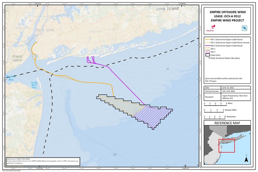
Exponent Engineering P.C.

Electrical Engineering and Computer
Science Practice
Ecological and Biological Sciences
Practice

Empire Offshore Wind:
Empire Wind Project (EW 1
and EW 2)

Offshore Electric- and
Magnetic-Field Assessment

Empire Offshore Wind: Empire Wind Project (EW 1 and EW 2) Offshore Electric- and Magnetic- Field Assessment Prepared for Empire Offshore Wind LLC 120 Long Ridge Road #3E01 Stamford, Connecticut CT 06902 Prepared by Exponent 17000 Science Drive Suite 200 Bowie, Maryland 20715 June 30, 2021 Exponent, Inc. 1805604.EX1 - 7393
June 30, 2021

Contents

                                                                                       Page

List of Figures                                                                         iv

List of Tables                                                                           v

Acronyms and Abbreviations                                                              vi

Executive Summary                                                                      viii

Introduction                                                                             1
    Project Description                                                                  1
    Magnetic Fields and Electric Fields                                                  3
    Assessment Criteria                                                                  4
      Human Exposure                                                                     4
      Marine Species Exposure                                                            5

Cable Configurations                                                                     6

Calculated Magnetic and Electric Fields                                                  8
    Calculated Magnetic-Field Levels                                                     8
    Calculated Electric-Field Levels Induced in Seawater                                10
    Calculated Electric-Field Levels Induced in Fish                                    11

Evaluation of EMF Exposure for Finfish Species in the Project Area                      12
    Description of Important Finfish Species Residing in the Project Area               13
      Behavioral Effects of Exposure to EMF from 50- and 60-Hz AC Sources               16
      Field Studies that Address Effects of Submarine Cables on Finfish Distribution    18
      Electrosensitivity in Sturgeon Species                                            19
    Evaluation of EMF Exposure from Project Cables                                      20

Evaluation of EMF Exposure for Elasmobranchs in the Project Area                        22
    Description of Elasmobranch Species Residing in the Project Area                    22
      Evidence of Magnetosensitivity and Electrosensitivity in Elasmobranchs            23
      Field Studies that Address Effects of Submarine Cables on Elasmobranch
      Distributions                                                                     24

1805604.EX1 - 7393                              ii
June 30, 2021

    Evaluation of EMF Exposure from the Project Cables                                  25

Evaluation of EMF Exposure for Large Invertebrates in the Project Area                  27
    Evidence of Magnetosensitivity in Large Marine Invertebrates                        28
    Evaluation of EMF Levels Produced by the Project Cables                             31

Evaluation of Chronic EMF Exposure for Finfish at Protective Coverings                  32
    Evaluation of EMF Levels at Areas with Protective Coverings                         34

Conclusions                                                                             35

References                                                                              37

Limitations                                                                             42

Attachment A         Cable Configurations
Attachment B         Calculation Methods
Attachment C         Calculated Magnetic- and Electric-Field Levels for Modeled Cable
                     Configurations

1805604.EX1 - 7393                              iii
June 30, 2021

List of Figures

                                                                                                  Page

Figure 1.            Overview of the proposed Lease Area and submarine export cable routes.          2
Figure 2.            Calculated magnetic-field levels in seawater above the submarine export
                     cable for 4-ft (1.2-m) burial depth and average loading.                        9

1805604.EX1 - 7393                                     iv
June 30, 2021
List of Tables
Page
Table 1. Calculated magnetic-field levels (mG) at a height of 3.3 ft (1.0 m) above the
seabed for a 4-ft (1.2-m) burial depth and average loading 10
Table 2. Calculated electric-field levels (mV/m) induced in seawater at a height of
3.3 ft (1.0 m) above the seabed for a 6.6-ft (2-m) burial depth and average
loading 11
Table 3. Calculated electric-field levels (mV/m) induced in electrosensitive marine
organisms at a height of 3.3 ft (1.0 m) above the seabed for a 4-ft (1.2-m)
burial depth and average loading 11
Table 4. Key demersal and benthopelagic fish species expected to inhabit the Project
Area (size at maturity = size at which 50% of species are reproductively
mature; common length = most frequent length within a species’ population) 13
Table 5. Key pelagic species expected to inhabit the Project Area (size at maturity =
size at which 50% of species are reproductively mature; common length =
most frequent length within a species’ population) 15
Table 6. Calculated maximum magnetic field (mG) and induced electric field for
peak loading at 3.3 ft (1.0 m) above the seabed based on proposed cable
configurations for the Project 21
Table 7. Elasmobranch species expected to utilize the Project Area (size at maturity =
size at which 50% of species are reproductively mature; common length =
most frequent length within a species’ population) 22
Table 8. Calculated maximum magnetic field (mG) and induced electric field for
peak loading at 3.3 ft (1.0 m) above the seabed based on proposed cable
configurations for the Project 26
Table 9. Important crustacean, bivalve, and squid species expected to inhabit the
Project Area 28
1805604.EX1 - 7393 vJune 30, 2021 Acronyms and Abbreviations µV/m Microvolts per meter A Ampere AC Alternating current ASFMC Atlantic States Fisheries Commission BOEM Bureau of Energy Ocean Management DC Direct current EMF Electric and magnetic fields Empire Empire Offshore Wind LLC EW Empire Wind ft Feet G Gauss HDD Horizontal directional drilling Hz Hertz ICES International Committee on Electromagnetic Safety ICNIRP International Commission on Non-Ionizing Radiation IEEE Institute of Electrical and Electronics Engineers km Kilometer kV Kilovolt Lease Area designated Renewable Energy Lease Area OCS-A 0512 m Meter MAFMC Mid-Atlantic Fishery Management Council mG Milligauss mi Statute miles mm Millimeter mT Millitesla mV/m Millivolts per meter MRE Marine Renewable Energy MW Megawatt NEFMC New England Fishery Management Council Nysted Nysted Wind Farm in Denmark 1805604.EX1 - 7393 vi
June 30, 2021

nm                   Nautical mile
NOAA                 National Oceanic and Atmospheric Administration
OD                   Outer diameter
POI                  Point of Interconnection
Project              The offshore wind project for OCS A-0512 proposed by Empire Offshore
                     Wind LLC consisting of Empire Wind 1 (EW 1) and Empire Wind 2 (EW
                     2).
Project Area         The area associated with the build out of the Lease Area, submarine
                     export cables, interarray cables, and all onshore Project facilities.
ROW                  Right-of-way
XLPE                 Cross linked polyethylene

1805604.EX1 - 7393                              vii
June 30, 2021 Executive Summary Empire Offshore Wind LLC (Empire) proposes to construct and operate an offshore wind facility in the designated Renewable Energy Lease Area OCS-A 0512 located approximately 14 statute miles (mi) (12 nautical miles [nm], 22 kilometers [km]) south of Long Island, New York, and 19.5 mi (16.9 nm, 31.4 km) east of Long Branch, New Jersey. Empire proposes to develop the Lease Area with two wind farms, known as Empire Wind 1 (EW 1) and Empire Wind 2 (EW 2) (collectively referred to hereafter as the Project). At the request of Empire, Exponent calculated the magnetic fields and induced electric fields associated with the operation of the submarine export cables that will transport electricity generated by the Project to shore. Field levels were calculated for the interarray cables connecting wind turbine generators to offshore substations, and for the offshore portion of submarine export cables connecting offshore substations to landfall locations in Brooklyn, New York, and Long Beach and Hempstead, New York. The purpose of the report is to describe the weak magnetic fields and weak electric fields induced in nearby seawater and marine organisms and to compare the calculated levels to those reported in the literature for potential effects on key marine species that inhabit the vicinity of the Project. The calculated field levels also are compared to exposure criteria for the general public for reference. Calculated magnetic-field levels were below reported thresholds for effects on the behavior of magnetosensitive marine organisms. Levels of electric fields induced in seawater and large fishes also were calculated to be below reported detection thresholds of local electrosensitive marine organisms. In addition, calculated magnetic-field levels in seawater were far below limits published by the International Committee on Electromagnetic Safety and the International Commission on Non-Ionizing Radiation designed to protect the health and safety of the general public. Note that this Executive Summary does not contain all of Exponent’s technical evaluations, analyses, conclusions, and recommendations. Hence, the main body of this report is at all times the controlling document. 1805604.EX1 - 7393 viii
June 30, 2021

Introduction

Project Description

Empire Offshore Wind LLC (Empire) proposes to construct and operate the Project located in
the designated Renewable Energy Lease Area OCS-A 0512 (Lease Area). The Lease Area
covers approximately 79,350 acres (32,112 hectares) and is located approximately 14 statute
miles (mi) (12 nautical miles [nm], 22 kilometers [km]) south of Long Island, New York, and
19.5 mi (16.9 nm, 31.4 km) east of Long Branch, New Jersey. Empire proposes to develop the
Lease Area with two wind farms, known as Empire Wind 1 (EW 1) and Empire Wind 2 (EW 2)
(collectively referred to hereafter as the Project). Both EW 1 and EW 2 are covered in this
Construction and Operations Plan (COP). EW 1 and EW 2 will be electrically isolated and
independent from each other. Each wind farm will, independently of one another, connect via
offshore substations to Points of Interconnection (POI) at onshore locations by way of export
cable routes and onshore substations. In this respect, the Project includes two onshore locations
in New York, where the renewable electricity generated will be transmitted to the electric grid.
The EW 1 Project will connect to the existing Gowanus POI in Brooklyn, New York. The EW 2
Project will connect to the existing Oceanside POI in Hempstead, New York. An overview of
the Project is shown in Figure 1. For EW 1 and EW 2, the renewable electricity generated will
be carried over alternating current (AC) interarray cables at a voltage of 66 kilovolts (kV) to an
offshore substation where it will be converted to 230 kV, and then carried to shore via
submarine export cables. This report summarizes the calculated levels of AC magnetic fields
and induced electric fields for the interarray and submarine export cables in the offshore portion
of the Project. It also provides a detailed assessment of magnetic fields and induced electric
fields in marine species in the proposed Project Area. The locations and routes of the interarray
and submarine export cables will differ among EW 1 and EW 2, but the calculations provided
are representative of both EW 1 and EW 2.

1805604.EX1 - 7393                               1
June 30, 2021

Figure 1.            Overview of the proposed Lease Area and submarine export cable routes.

1805604.EX1 - 7393                                                   2
June 30, 2021

The assessment of the onshore export and interconnection cables connecting the Project to
existing POIs is provided in a companion report titled Empire Offshore Wind: Empire Wind
Project (EW 1 and EW 2) - Onshore Electric and Magnetic Field Assessment.

Magnetic Fields and Electric Fields

The flow of electric currents in the submarine export and interarray cables will be new sources
of magnetic fields in the marine environment. These magnetic-field levels will be highest at the
cables’ surface and decrease rapidly with distance, generally in proportion to the square of the
distance from the cables. Magnetic fields are reported as root-mean-square flux density in units
of milligauss (mG), where 1 Gauss is equal to 1,000 mG. 1

The submarine export cables also are a source of electric fields inside the cable insulation and
armoring due to the voltage applied to the conductors located within the cables. However, since
the conductors are encased within the cables with grounded metallic sheathing and the cable is
covered with steel armor, these electric fields do not enter the marine environment because they
are entirely blocked by this shielding (CSA Ocean Sciences Inc. and Exponent, 2019).

The oscillating magnetic field produced by the cables, however, will induce a weak electric field
in the marine environment and in marine species near the cables. Since the electric field is
induced by the cables’ magnetic field, it will vary depending on the flow of electric currents in
the cables, rather than voltage. Similar to magnetic fields, the induced electric fields decrease
rapidly with distance from the cables. Induced electric fields are reported in units of millivolts
per meter (mV/m).

The levels of both magnetic fields and induced electric fields will vary depending on the
magnitude of the electric current—reported in units of Ampere (A)—carried on the cables at
any one time. Therefore, calculations of magnetic fields represent only a snapshot at one
moment due to the varying power generated by the turbines, which depends both on operational
status and wind speed. To account for the variability of current, calculations of magnetic fields
were performed for the peak current at which the windfarm can operate, which will indicate the

1
    Magnetic fields also are commonly reported in units of microtesla, where 0.1 microtesla is equal to 1 mG.

1805604.EX1 - 7393                                       3
June 30, 2021 highest magnetic-field levels that can occur, and for the annual average current that represents more typical field levels over time. Additional discussion of the fields associated with offshore windfarm submarine cables in general is provided in a 2019 report issued by the Bureau of Ocean Energy Management (CSA Ocean Sciences Inc., and Exponent, 2019). Assessment Criteria Human Exposure While the likelihood of persons coming in close proximity to the undersea cables is minimal and limited to those who might be scuba diving at the seabed, the level of potential exposure was still considered. There are no federal standards that limit either magnetic or electric fields produced by transmission infrastructure, but two international organizations provide guidance on limiting exposure to magnetic fields, which is based on extensive review and evaluations of relevant research of health and safety issues—the International Committee on Electromagnetic Safety (ICES), which is a committee under the oversight of the Institute of Electrical and Electronics Engineers, and the International Commission on Non-Ionizing Radiation (ICNIRP), an independent organization providing scientific advice and guidance on electromagnetic fields. Both organizations have recommended limits designed to protect health and safety of persons in occupational settings and for the general public. The ICES maximum permissible exposure limit for the general public to 60-Hertz (Hz) magnetic fields is 9,040 mG, and ICNIRP determined a reference level limit for whole-body exposure to 60-Hz magnetic fields at 2,000 mG (ICES, 2002/2005, ICNIRP, 2010). The World Health Organization (WHO) views these standards as protective of public health (WHO, 2007). As the WHO (2019) also states on its website, “[b]ased on a recent in-depth review of the scientific literature, the WHO concluded that current evidence does not confirm the existence of any health consequences from exposure to low level electromagnetic fields.” 1805604.EX1 - 7393 4
June 30, 2021

Marine Species Exposure

Some marine species have specialized electro-sensory receptors that enable them to detect
electric fields or magnetic fields, or both, so fields from undersea cables are of ecological
interest. Generally, marine species that have these specialized receptors can detect electric fields
and magnetic fields over a limited frequency range (CSA Ocean Sciences Inc. and Exponent,
2019):

     •     The earth’s geomagnetic field (i.e., a static field at a frequency of approximately 0 Hz);

     •     The approximately 0-Hz electric fields created by ocean currents;

     •     The induced electric field created by fish movements in the earth’s geomagnetic field;
           and

     •     Electric fields produced by biological functions of fish with frequencies from 0 to
           approximately 10 Hz (Bedore and Kajiura, 2013).

While some species are capable of detecting fields at these lower frequencies in the natural
environment, the electric and magnetic fields from the AC cables associated with the Project
oscillate at a much higher frequency—60 Hz. Therefore, this assessment has focused on 50/60
Hz fields from AC submarine cables. A detailed assessment of magnetic fields and induced
electric fields in marine species in the proposed Project Area is included in later sections of this
report.

1805604.EX1 - 7393                                  5
June 30, 2021
Cable Configurations
Exponent calculated the 60-Hz magnetic and induced electric fields from the submarine export
and interarray cables proposed to be installed as part of the Project. These values were
compared to assessment criteria to assess potential effects on marine species. Detailed
descriptions of the cable configurations are provided in Attachment A, and description of the
calculation methods is provided in Attachment B. A brief summary of each is provided below.
The proposed submarine cables consist of up to 260 nm of 66-kV AC 2 interarray cables and 66
nm of 230-kV AC submarine export cables, including up to 40 nm for EW 1 and up to 26 nm
for EW 2. Cables are expected to be buried at least 6 feet (ft, 1.8 meters [m]) beneath the seabed
. Calculations were performed at 4 ft (1.2 m) burial depth, resulting in higher field levels than
where the cables are buried deeper. 3 Where it is impossible to bury a cable, it will be laid on the
seabed and covered with rock berm or other protective covering with a minimum coverage of
3.3 ft (1 m) for the submarine export cable and 2.3 ft (0.7 m) for the interarray cable. At
landfall, the submarine export cable at EW 2 will be installed via horizontal directional drilling
(HDD) with a minimum horizontal distance between the two submarine export cables of 33 ft
(10 m) and minimum burial depth of 6.0 ft (1.8 m). At EW 1, the submarine export cables will
be installed via open-cut trench or HDD, with a minimum burial depth of 6.0 ft (1.8 m), except
for a short (less than 30.0 ft [9.1 m]) protected duct installation where the protective covering
will decrease to a minimum depth of 1 ft (0.3 m) at the transition to HDD. For either HDD or
open cut trench installation, the expected burial depth for the vast majority of the installation
will be much greater than the 1 ft (0.3 m) modeled and so field levels would be lower than
calculated herein.
Magnetic- and induced electric-field levels were calculated for each of these cable
configurations using minimum target burial depths and conservative assumptions to ensure that
2
Some other submarine cables, such as those primarily investigated by Hutchison et al., (2018) operate using
direct current (DC) transmission lines
3
Empire has refined the Project Design Envelope since this assessment was completed and is no longer
considering a 4 ft (1.2 m) burial depth along the submarine export cable routes.
1805604.EX1 - 7393 6June 30, 2021 the calculated field levels would overestimate the field levels that would be measured at any specified loading. Note that all indicated burial depths are specified to the top of the cable. 1805604.EX1 - 7393 7
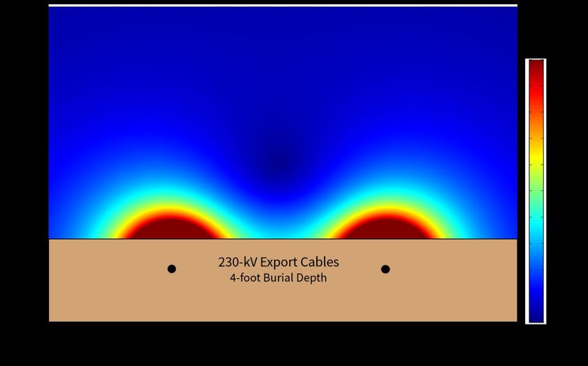
June 30, 2021

Calculated Magnetic and Electric Fields

Magnetic-field and induced electric-field levels were calculated for each of the proposed
submarine export and interarray cable configurations for buried, surface-laid, and landfall
installation types. Field levels were calculated for average and peak loading, and for locations at
the seabed and at a height of 3.3 ft (1.0 m) above the seabed. The calculated field levels at 3.3 ft
(1.0 m) above the seabed for a 4-ft (1.2 m) burial depth and average loading are summarized
below.

Calculated magnetic-field levels are summarized and compared to limits on human exposure
below. Calculated induced electric-field levels are summarized below and compared to relevant
detection thresholds for marine species in subsequent sections of this report. Calculated field
levels for all modeled cable configurations are provided in Attachment C.

Calculated Magnetic-Field Levels

Calculated magnetic-field levels are plotted in Figure 2 for the submarine export cable and
summarized in Table 1 for both the submarine export cable and interarray cable for a 4-ft
(1.2 m) burial depth and average loading. The highest calculated magnetic-field level at a height
of 3.3 ft (1.0 m) above the seabed is 35 mG for the submarine export cable and 16 mG for the
interarray cable. Field levels decrease rapidly with distance, falling to less than 3 mG beyond a
horizontal distance of 30 ft (9.1 m) from either cable type. All calculated field levels are well
below the ICNIRP reference level of 2,000 mG and the ICES maximum permissible exposure
limit of 9,040 mG for exposure of the general public.

1805604.EX1 - 7393                               8
June 30, 2021

Where the cables are surface-laid for short distances and covered with protective rock berm or
other protective covering, or where the submarine export cable burial depth may decrease for
short distances approaching landfall, the field levels would be higher than summarized above.
Field levels would also be higher for peak loading on the cables. 4 These higher field levels,
however, would occur for short distances along the route and for short periods of time at peak
loading. Conversely, where the cables are installed even further than 4 ft below the seabed, the
magnetic- and induced electric-field levels will be lower than modeled. The magnetic-field
levels for all burial depths and loading levels would decrease rapidly with distance from the
cables and would be well below the ICNIRP and ICES limits for exposure of the general public.

Figure 2.            Calculated magnetic-field levels in seawater above the submarine export cable
                     for 4-ft (1.2-m) burial depth and average loading.

4
    The highest calculated magnetic field for any configuration at the seabed was 1,237 mG at average loading and
    1,455 mG at peak loading. These field levels decrease very rapidly to 22 mG and 26 mG, respectively, at a ±10
    ft (±3 m) horizontal distance from the cable. At a height of 3.3 ft (1.0 m) above the seabed, the highest
    calculated magnetic-field level was 98 mG at average loading and 116 mG at peak loading. All these maxima
    are calculated above the submarine export cable at landfall and are expected to apply only to a short (less than
    30 ft [9.1 m]) distance along the route.

1805604.EX1 - 7393                                        9
June 30, 2021
Table 1. Calculated magnetic-field levels (mG) at a height of 3.3 ft (1.0 m) above the
seabed for a 4-ft (1.2-m) burial depth and average loading
Horizontal Distance from the Cable
±10ft ±30 ft
Max
(±3 m) (±9.1 m)
Submarine Export Cable* 35 14 2.8
Interarray Cable 16 5.9 1.0
* The submarine export cable includes two cables side-by-side. The horizontal distance
is measured outward from nearest cable.
Calculated Electric-Field Levels Induced in Seawater
Calculated electric-field levels induced in seawater are summarized in Table 2 for the submarine
export cable and interarray cable for a 4-ft (1.2-m) burial depth and average loading. The
highest calculated field levels at a height of 3.3 ft (1.0 m) above the seabed are 2.4 mV/m for the
submarine export cable and 1.0 mV/m for the interarray cable. Where the cables may be
surface-laid for short distances, or where the burial depth may decrease for short distances (for
example approaching landfall), the field levels would be higher. Field levels would also be
higher at peak cable loading. 5 These higher field levels, however, would occur for short
distances along the route and for short periods of time. Conversely, where the cables are
installed even further than 4 ft (1.2 m) below the seabed, the magnetic- and induced electric-
field levels will be lower than modeled. As for all modeled cable configurations, field levels
would decrease rapidly with distance. For horizontal distances beyond 30 ft (9.1 m) from the
cables, the induced electric-field levels were calculated to be less than 1.0 mV/m for both cable
configurations at average and peak loading.
5
The highest calculated electric field induced in seawater for any configuration at the seabed was 14 mV/m at
average loading and 16 mV/m at peak loading. These field levels decrease very rapidly to 2.2 mV/m and
2.5 mV/m, respectively, at a ±10 ft (±3 m) horizontal distance from the cable. At a height of 3.3 ft (1.0 m)
above the seabed the highest calculated electric-field level in seawater was 3.8 mV/m at average loading and 4.5
mV/m at peak loading. All these maxima are calculated above the submarine export cable at landfall and are
expected to apply only to a short (less than 30 ft [9.1 m]) distance along the route.
1805604.EX1 - 7393 10June 30, 2021
Table 2. Calculated electric-field levels (mV/m) induced in seawater at a height of 3.3 ft
(1.0 m) above the seabed for a 6.6-ft (2-m) burial depth and average loading
Horizontal Distance from the Cable
Max ±10 ft (±3 m) ±30 ft (±9.1 m)
Submarine Export Cable* 2.4 1.7 0.8
Interarray Cable 1.0 0.6 0.2
* The submarine export cable includes two cables side-by-side. The horizontal distance is measured
outward from the nearest cable.
Calculated Electric-Field Levels Induced in Fish
In addition to induced electric fields in seawater, the oscillating magnetic field also will induce
an electric field within the body of a marine organism. The strength of the electric field induced
in an object like a fish, however, depends upon the size (length and girth) of the fish. As shown
in Table 3 below, the electric fields induced within large representative fish are about 10-fold
lower than the electric field induced in seawater. The calculated electric fields induced in
electrosensitive marine organisms at a height of 3.3 ft (1.0 m) above the seabed are summarized
in Table 3 for the submarine export cable and interarray cable for a 4-ft (1.2-m) burial depth and
average loading. The calculated electric-field levels induced in marine organisms are 0.4 mV/m
or less. Electric-field levels induced in marine organisms would be higher for short distances
along the route where burial depth decreases and for short periods at increased loading. 6
Calculated field levels decrease rapidly with distance, falling to less than 0.05 mV/m for
horizontal distances beyond 30 ft (9.1 m) from the cables for all cable configurations for both
average and peak loading.
Table 3. Calculated electric-field levels (mV/m) induced in electrosensitive marine
organisms at a height of 3.3 ft (1.0 m) above the seabed for a 4-ft (1.2-m) burial
depth and average loading
Dogfish Sturgeon
Submarine Export Cable 0.2 0.4
Interarray Cable 0.1 0.2
6
The highest calculated electric field induced in marine organisms for any configuration at the seabed was
15 mV/m at average loading and 18 mV/m at peak loading. These field levels decrease very rapidly to
0.3 mV/m or less at a ±10 ft (±3 m) horizontal distance from the cable. At a height of 3.3 ft (1.0 m) above the
seabed the highest calculated electric-field level in seawater was 1.2 mV/m at average loading and 1.4 mV/m at
peak loading. All these maxima occurred in the Sturgeon and above the submarine export cable at landfall and
are expected to occur for only a short (less than 30 ft [9.1 m]) distance along the route.
1805604.EX1 - 7393 11June 30, 2021 Evaluation of EMF Exposure for Finfish Species in the Project Area A wide range of marine and freshwater fish species have been observed to exhibit magnetosensitivity; these include salmonids, tuna, herrings, carp, and mackerel. The ability to detect magnetic fields is theorized to be due to the presence of magnetite particles in the bones and organs of various species, the presence of which allows the fish to perceive small changes in the earth’s geomagnetic field (Hanson and Westerberg, 1987; Harrison et al., 2002; Tanski et al., 2011; Walker et al., 1998). Together with other environmental cues, such as water temperature, olfactory signals, current direction, current strength, and light, perceived changes in the geomagnetic field can be incorporated to guide fish migration between key habitats. It is important to note that the earth’s geomagnetic field (~0 Hz) has a frequency quite different from the magnetic field produced by 60-Hz AC submarine cables, so it is not possible to interpret responses of fish to AC cables from studies conducted with static fields. However, given that specialized sensory mechanisms evolved in fish to take advantage of a common cue (the earth’s geomagnetic field) and occurs across a broad diversity of species, it is reasonable to assume that where responses to EMF have been observed, these would be similar to those for fish species that have not been studied. In addition to the ability to detect magnetic fields, a subset of fish species have developed specialized and sensitive electroreceptors (called ampullae of Lorenzini) that can detect low- level electric fields. Electrosensitive fish include sturgeon species (family Acipenseridae); these are primarily anadromous fish that move between freshwater, estuarine, and coastal environments along the Atlantic coast of the United States. Electrosensitive fish can detect and respond to the low-level bioelectric fields produced by prey, so this ability allows for optimized foraging. 1805604.EX1 - 7393 12
June 30, 2021

    Description of Important Finfish Species Residing in the Project
    Area

    The Project Area is within the known habitat and range of a number of commercially important
    finfish 7 species (listed in Table 4 and Table 5): many of these species are actively managed by
    governmental agencies to ensure population stability and sustainability. In terms of the potential
    for encountering cable associated EMF, bottom-dwelling (demersal) fish have been identified as
    the most likely to be exposed, since these species inhabit the portion of the water column closest
    to the cable (Bull and Helix, 2011). Conversely, fish that inhabit the upper portions of the water
    column (pelagic) are less likely to spend time within the area immediately above buried cables
    where the levels of EMF are higher. Additionally, highly mobile fish species with a large range
    also are more likely to inhabit regions distant from the cables, reducing the possibility of
    exposure to EMF from the Project cables. Hence, identified fish species have been categorized
    by behaviors and preferred habitats that are expected to affect the likelihood of encountering the
    cable route. Size information is provided in these tables as the magnitude of electric fields
    induced within fish scales with body size. Fish species of commercial importance that are
    managed and monitored by fisheries are identified as well.

Table 4.      Key demersal and benthopelagic fish species expected to inhabit the Project Area
              (size at maturity = size at which 50% of species are reproductively mature;
              common length = most frequent length within a species’ population)

                                                                                Size at            Size,        Managing
                                                                                maturity         common         Agency or
             Species                    Occurrence/Range/Habitat                 (cm)1         length(cm)1        FMC
Atlantic Butterfish (Peprilus      Schooling over the continental shelf in
                                                                                    12              20            MAFMC
triacanthus)                       waters 49 to 1380 (15 m to 420 m) deep
Atlantic Cod (Gadus morhua)        Shoreline to outer continental shelf             63                            NEFMC

                                   Over sandy and muddy bottoms from
Atlantic Croaker (Micropogonias
                                   coastal areas to 330 ft (100 m)                  18              30            ASFMC
undulates)

Atlantic Sturgeon (Acipenser       Nearshore areas with long migrations
                                                                                   190              250           ASFMC
oxyrinchus oxyrinchus)             into freshwater rivers
Black Sea Bass (Centropristis      Inhabits rock jetties and bottoms in
                                                                                   19.1             30            ASFMC
striata)                           shallow coastal waters

    7
        The term finfish is used to distinguish these species from the elasmobranchs, which are discussed in a separate
        section.

    1805604.EX1 - 7393                                        13
June 30, 2021
Size at Size, Managing
maturity common Agency or
Species Occurrence/Range/Habitat (cm)1 length(cm)1 FMC
In coastal areas over sandy and muddy
Black Drum (Pogonias cromis) NA 50 ASFMC
bottoms
Cunner (Tautogolabrus Inshore, shallow waters, frequently in 38 (max
NA
adspersus) large numbers around structures length)
Haddock (Melanogrammus Common over rock, gravel and shell
aeglefinus) substrate from 260 ft to 660 ft (80 to 35 35 NEFMC
200 m)
Monkfish (Lophius americanus) Throughout continental shelf 47 90 NEFMC
Ocean Pout (Zoarces Throughout continental shelf 110 (max
28.8 NEFMC
americanus) length)
Northern Kingfish (Menticirrhus Shallow coastal waters of an
NA 30
saxatilis) approximate 3.3-ft (10 m) depth
Northern Puffer (Sphoeroides Bays, inlets, estuaries and other
NA 20
maculatus) protected coastal waters
Northern Searobin (Prionotus On sandy bottoms between 49 ft and
NA 30
carolinus) 560 ft (15 m and 170 m) deep
Pollock (Pollachius virens) Inshore and offshore to >660 ft (200 m) 39.1 60 NEFMC
Red Hake (Urophycis chuss) Soft substrate in nearshore to a 430-ft
26 NA NEFMC
(130 m) depth
Silver Hake or Whiting Sandy bottoms in shallow areas and to
23 37 NEFMC
(Merluccius bilinearis) outer continental shelf
Smallmouth Flounder (Etropus On soft bottoms to depths of 300 ft
NA NA
microstomus) (91 m)
Spot (Leiostomus xanthurus) Associated with sandy or muddy
substrates in coastal waters to 200 ft NA 25 ASFMC
(60 m)
Spotted Hake (Urophycis regia) Common along the continental shelf at
depths between 360 ft and 600 ft (110 m NA 17
and 185 m)
Summer Flounder (Paralichthys Sandy substrates in mostly nearshore
28 NA MAFMC
dentatus) areas (usually to 120 [37 m])
Tautog (Tautoga onitis) Hard-bottom and reef habitats in waters
18 NA
to 250 ft (75 m) deep
Weakfish (Cynoscion regalis) In shallow waters to 85 ft (26 m) over
14 50
sandy and muddy substrates
White Hake (Urophycis tenuis) Muddy substrates from 330 ft to 820 ft
46 70 NEFMC
(100 m to 250 m)
Witch Flounder (Glyptocephalus Soft mud substrates usually between
30 NA NEFMC
cynoglossus) 150 ft and 1150 ft (45 m and 350 m)
Windowpane Flounder Sand substrates from nearshore to a
22 NA NEFMC
(Scophthalmus aquosus) 150-ft (45-m) depth
1805604.EX1 - 7393 14June 30, 2021
Size at Size, Managing
maturity common Agency or
Species Occurrence/Range/Habitat (cm)1 length(cm)1 FMC
Winter Flounder Muddy and hard substrate in depths of
(Pseudopleuronectes less than 460 ft (140 m) 27 NA NEFMC
americanus)
Yellowtail Flounder (Limanda Sand and mud substrates usually
ferruginea) between 100 ft and 295 ft (30 m and 30 NA NEFMC
90 m)
1
Information from fishbase.org; Size information is important for calculating fields induced within the body of a marine
animal and is discussed further in Attachment B.
Key: ASFMC – Atlantic States Fisheries Commission; MAFMC – Mid-Atlantic Fishery Management Council; NEFMC-
New England Fishery Management Council; NA – Not available
Table 5. Key pelagic species expected to inhabit the Project Area (size at maturity = size at
which 50% of species are reproductively mature; common length = most frequent
length within a species’ population)
Size,
Size at common
maturity length
Species Occurrence/Range/Habitat (cm)1 (cm)1 Managing Agency or FMC
Albacore Tuna (Thunnus In surface waters of depths of to 85 100 NOAA Fisheries, Atlantic Highly
alalunga) 2,000 ft (600 m) Migratory Species
Atlantic Bluefin Tuna Nearshore and offshore. 97 200 NOAA Fisheries, Atlantic Highly
(Thunnus thynnus) Migratory Species
Atlantic Herring (Clupea Open waters of depths between 17 30 NEFMC
harengus) 0 ft and 1190 ft (0 m and 364 m)
Atlantic Mackerel In surface waters over the 29 30 MAFMC
(Scomber scombrus) continental shelf
Atlantic Menhaden Forms large schools in coastal 18 NA ASFMC
(Brevoortia tyrannus) waters
Atlantic Skipjack Tuna Epipelagic, open ocean 40 80 NOAA Fisheries, Atlantic Highly
(Katsuwonus pelamis) Migratory Species
Atlantic Yellowfin Tuna Epipelagic, oceanic fish in 103 150 NOAA Fisheries, Atlantic Highly
(Thunnus albacares) upper 330 ft (100 m) Migratory Species
Bay Anchovy (Anchoa In shallow tidal areas, especially 4 6
mitchilli) those with brackish water and
muddy bottoms
Blueback Herring (Alosa In estuaries and coastal areas, NA 27.5
aestivalis) usually in schools
Bluefish (Pomatomus Nearshore to offshore 30 60 MAFMC
saltatrix)
Striped Anchovy (Anchoa In dense schools at the surface NA 11
hepsetus) of shallow coastal waters
1
Information from fishbase.org; Size information is important for calculating fields induced within the body of a marine
animal and is discussed further in Attachment B
Key: ASFMC – Atlantic States Fisheries Commission; MAFMC – Mid-Atlantic Fishery Management Council; NEFMC
– New England Fishery Management Council; NOAA – National Oceanic and Atmospheric Administration; NA – Not
available
1805604.EX1 - 7393 15June 30, 2021 Although a large number of studies have been conducted to assess the sensitivity and behavioral responses of various fish species to static magnetic fields, relatively fewer investigations have been conducted with AC magnetic fields. Furthermore, when such studies have been conducted, many have focused on low frequency fields (i.e., 10 Hz or less), as these are common in the natural marine environment. Therefore, scientists have summarized the available information regarding the ability of finfish to detect AC magnetic fields and used it to predict the general responses of magnetosensitive fish based on the observation that magnetosensitivity in finfish developed to detect a common signal, the geomagnetic field. Much of the information on fish detection and response thresholds has been assessed in laboratory studies, which can be categorized into those evaluating physiological effects on fish following long-term (>24 hours) exposure to AC EMF, and those that examine the effect of such fields on the immediate behavior of individual adult fish. Since the majority of fish are expected to experience only transitory exposure to the Project cables, the first group of studies is of limited relevance. Behavioral Effects of Exposure to EMF from 50- and 60-Hz AC Sources The bulk of the scientific literature generated from laboratory studies does not indicate that 50- or 60-Hz fields have adverse effects on adult finfish behavior and orientation. Richardson et al. (1970) exposed both Atlantic salmon (Salmo salar) and American eel (Anguilla rostrata) to a 500 mG magnetic field produced by a 60-75-Hz AC power source. Exposed fish exhibited no change in swim behaviors, leading the study authors to conclude that, under field conditions, EMF produced by 60-Hz AC cables is not likely to alter the behavior or activity of either species (Richardson et al., 1970). More recently, the Marine Scotland Science Agency also assessed European eel (A. anguilla) and Atlantic salmon behavior in response to high frequency magnetic fields, produced by a 50- Hz AC power source. Atlantic salmon were exposed to magnetic-field strengths between 1.3 and 950 mG, during which no significant change in salmon swimming or behavior was noted (Armstrong et al., 2015). Similarly, European eel were exposed to a 50-Hz AC power source that produced a magnetic field of 960 mG. Researchers observed no effects of magnetic-field exposure on eel swim behavior, orientation, or passage through tank system (Orpwood et al., 2015). Overall, studies conducted by Richardson et al. (1970), Armstrong et al. (2015), and 1805604.EX1 - 7393 16
June 30, 2021

Orpwood et al. (2015) demonstrate that 50-75 Hz AC cables do not alter the behavior of either
salmon or eel under controlled laboratory conditions, indicating that magnetic fields produced
by these power sources are not readily detected by these magnetosensitive migratory fish
species.

The effects of magnetic fields produced by 60-Hz AC power sources were also assessed for a
series of freshwater fish species, including pallid sturgeon (Scaphirhynchus albus), largemouth
bass (Micropterus salmoides), and redear sunfish (Lepomis microlophus), at the U.S.
Department of Energy’s Oak Ridge Laboratory. Fish were exposed to magnetic fields produced
by an AC electromagnet and changes in behavioral and orientation were observed. During
exposure to a 1,657,800 mG magnetic field, redear sunfish were observed to significantly prefer
shelters nearest to the magnetic-field source (Bevelhimer et al., 2013). Once removed from the
magnetic field, however, redear sunfish resumed normal distribution within the tank, indicating
that once removed from the produced field, normal behavior was re-established. The authors
also reported no long-term effect on fish health resulting from the exposure to this high-strength
field (Bevelhimer et al., 2013). When largemouth bass were exposed to a 24,500 mG magnetic
field from a 60-Hz AC power source, researchers observed no significant changes in fish
behavior or swimming, leading to the conclusion that “the evidence from this study does not
support an effect on free-swimming largemouth bass … from EMF delivered at an intensity that
would be expected from a power transmission cable” (Bevelhimer et al., 2015, p. 12). Pallid
sturgeon were exposed to magnetic fields from a 60-Hz AC power source, using a more
complex laboratory mesocosm apparatus (Bevelhimer et al., 2015). Researchers observed that
magnetic fields strengths of approximately 18,000 to 24,500 mG had no effect on sturgeon
behavior or positioning within the tanks suggesting that magnetic fields of these strengths are
not detected by sturgeon (Bevelhimer et al., 2015).

In summary, the scientific literature evaluated here demonstrates that magnetosensitive fish do
not readily detect or alter their behavior in response to magnetic fields produced by 50/60Hz AC
cables. Moreover, even when the field is high enough for fish to detect (i.e., over
1,000,000 mG), effects are minor and reversible once fish move away from the magnetic field.

1805604.EX1 - 7393                              17
June 30, 2021

Field Studies that Address Effects of Submarine Cables on Finfish
Distribution

In addition to controlled laboratory studies, field surveys of finfish distributions at submarine
cables sites can provide important data on the in situ effects of AC EMF on local populations of
fish. These types of surveys include those conducted specifically at marine AC cables sites and
those conducted at offshore wind farm sites where generated power is transmitted to shore by
AC submarine cables.

Between 2012 and 2014, researchers at the Marine Science Institute at the University of
California, Santa Barbara, and BOEM tracked fish populations at both energized and
unenergized 60-Hz submarine cables off the California coast. Measured magnetic fields at
energized cable sites ranged between 730 to 1,100 mG (Love et al. 2016). Over the three years,
more than 40 different fish species were observed, including demersal California halibut
(Paralichthys californicus), sanddab (Citharichthys sordidus), and seaperch (Sebastes spp). No
differences, however, were identified between fish communities observed at the energized
versus unenergized cable routes. While the physical structure of the unburied cables attracted a
higher density of fish when compared to natural sediment bottoms (“reef effect”), the presence
of magnetic fields produced by the cable had no attractive or repulsive effect on resident fish
(Love et al. 2016). Thus, the results of this survey indicate that the magnetic fields produced by
an AC cable do not alter fish distributions or behavior.

Similarly, multiple studies have been conducted at many established offshore wind farm sites
that use 50/60 Hz AC transmission cables to conduct generated energy on shore; results from
these studies overwhelmingly demonstrate that the presence of wind farms and operating cables
have no effect on resident fish populations. For example, at the Horns Rev Offshore Wind Farm
site near Denmark, nearly 10 years of pre- and post-construction biological population data were
collected, including data on species similar to those expected to inhabit the Project Area such as
various flounder and flatfish species. Evaluation of all collected population data at this site
demonstrated that there were “no general significant changes in the abundance or distribution
patterns of pelagic and demersal fish” (Leonhard et al., 2011). For reef-associated species,
increased abundance was noted around turbine footings, which were concluded to be a result of
the vertical structure provided by footings.

1805604.EX1 - 7393                               18
June 30, 2021

Similarly, at the Wolfe Island Wind Farm site in Lake Ontario, multiple survey methods were
used to track changes in fish populations; results of these surveys led researchers to conclude
that there was “little to no effect of the Wolfe Island submarine cable on local fish
communities” (Dunlop et al., 2016). Following the construction of Thorntonbank Wind Farm in
Belgium, some short-lived changes in the abundance of certain fish and invertebrate species
were observed; however, the temporary nature of these alterations strongly indicate that the
changes were not related to the cable’s magnetic fields (Vandendriessche et al., 2015).

Conversely, some minor potential effects on fish distributions—termed “asymmetries in the
catches”—were observed along the Project cables of the Nysted Wind Farm in Denmark
(Nysted) (Vattenfall and Skov-og, 2006). In contrast to other surveys, however, baseline fish
population data were not collected at the Nysted site, complicating the interpretation of these
data. Moreover, the energy loading of the Nysted cable did not correlate with measures of fish
distribution, indicating that EMF levels were not the source of differences in distributions and
that the cable did not act as a barrier to fish movement, with the possible exception of flounder
(Vattenfall and Skov-og, 2006). The authors theorized, however, that the physical conditions of
the seabed along the cable route may explain the reactions in flounder.

Overall, the various population studies conducted at either submarine AC cable sites or offshore
wind farm sites show that 50/60 Hz magnetic fields do not affect fish distributions. As such, the
results of these surveys agree with the findings of the laboratory studies that demonstrate no
significant population-level distributional or behavioral effects of AC EMF on fish species.

Electrosensitivity in Sturgeon Species

Comparatively few fish species are capable of detecting electric fields in addition to magnetic
fields. The endangered Atlantic sturgeon, which inhabits the Project Area, is one of these fish
species. Given this, the ability of sturgeon to detect electric fields associated with 50/60-Hz
power sources was evaluated in the scientific literature. Basov (1999) exposed two different
sturgeon species—sterlet (Acipenser ruthenus) and Russian sturgeon (Acipenser
gueldenstaedtii)—to 50-Hz AC electric fields at intensities between 20 to 60 mV/m and
observed how fish responded to these (Basov,1999). The lower 20 mV/m level induced minor
alterations in fish orientation and also increased search and foraging behaviors in the vicinity of

1805604.EX1 - 7393                              19
June 30, 2021

the power source. This indicates that small-scale behavior effects may occur in electrosensitive
sturgeon exposed to electric-field intensities of 20 mV/m at 50/60 Hz.

Evaluation of EMF Exposure from Project Cables

The magnetic fields calculated from cable configurations and burial depths proposed for the
Project Area are presented in Table 6. At peak loading, magnetic-field levels were calculated to
be 41 mG at a 3.3 ft (1 m) distance from the seabed directly over the cable. This value is about
12 times lower than the 500 mG magnetic field that was demonstrated to have no behavioral
effects on either Atlantic salmon or American eel. Field strengths associated with significant
changes in fish behavior are orders of multiple magnitude higher (i.e., 1,657,800 mG for redear
sunfish) than those expected at the Project cables. These studies of multiple fish species indicate
that the magnetic fields produced by the Project cables will be below the level of detection for
marine finfish species.

In addition to magnetic-field levels, induced electric-field strengths, based on an Atlantic
sturgeon model, were calculated (Table 6). The Atlantic sturgeon was selected as a model
species due to their electrosensitivity, and the sturgeon were modeled as an ellipsoid 6 ft (1.8 m)
in length and a maximum girth of 2.5 ft (0.8 m). 8 The maximum value at 3.3 ft (1.0 m) above
the buried cables (0.5 mV/m) is projected to occur along the submarine export cable. This
maximum calculated induced electric-field strength is 40 times lower than the 20 mV/m electric
field reported as the threshold for changes in behavioral Russian sturgeon and sterlet, 20 mV/m
(Basov et al., 1999). Modeled induced electric fields in seawater also are predicted to be below
this reported detection threshold level (Table 6).

Subsequently, the scientific literature summarized above does not indicate that EMF from the
Project cables would be detectable by resident magnetosensitive and electrosensitive finfish
species, including the federally endangered Atlantic sturgeon and shortnose sturgeon. Because
of this, the operating cables therefore are not expected to adversely affect the populations or
distributions of finfish in the Project Area.

8
    Girth was determined using a standard length-girth-weight relationship for the related lake sturgeon
    (http://files.dnr.state.mn.us/areas/fisheries/baudette/lksweight.pdf).

1805604.EX1 - 7393                                       20
June 30, 2021
Table 6. Calculated maximum magnetic field (mG) and induced electric field for peak
loading at 3.3 ft (1.0 m) above the seabed based on proposed cable
configurations for the Project
Induced Electric Field (mV/m)
Magnetic
Cable Type Burial Depth Field (mG) Seawater Sturgeon Model
Submarine Export Cable 4 ft (1.2 m) 41 2.8 0.5
Interarray cable 4 ft (1.2 m) 20 1.2 0.3
1805604.EX1 - 7393 21June 30, 2021
Evaluation of EMF Exposure for Elasmobranchs in the
Project Area
Cartilaginous fish, like skates, sharks, and rays, are referred to collectively as elasmobranchs;
these species are common in coastal and oceanic environments. Elasmobranchs, as a group, are
both magnetosensitive and electrosensitive. Several species have been documented to utilize
alterations in the geomagnetic field to direct movement and migration, and the ability to detect
low frequency bioelectric fields (generally between 1 and 10 Hz) allows predators to locate prey
via the low frequency electric fields they produce (Bedore and Kajiura, 2013).
Description of Elasmobranch Species Residing in the Project
Area
A number of different elasmobranch species are expected to inhabit the Project Area, including
at least 13 different shark, skate, and dogfish species (Table 7). Individual species are expected
to utilize this area at different rates: smaller demersal species like skates and dogfish tend to
have smaller ranges, constrained to coastal areas, while large pelagic shark species may be
migratory with ranges of hundreds of kilometers (Vandeperre et al., 2014). For pelagic species,
the Project Area represents only a tiny proportion of the total marine habitat, while the localized
populations of the smaller, demersal elasmobranch species may more frequently encounter
submarine export cable routes. Hence, elasmobranchs have been categorized according to these
groups, as shown in Table 7.
Table 7. Elasmobranch species expected to utilize the Project Area (size at maturity =
size at which 50% of species are reproductively mature; common length =
most frequent length within a species’ population)
Size,
Size at common
Habitat Species Occurrence/Range/Habitat maturity (cm)1 length (cm)1
Clearnose Skate (Raja From bays and estuaries to depths
49 NA
eglanteria) of up to 330m
Little Skate (Leucoraja On sand and gravel substrates to
32 NA
erinacea) water depths to 90m
Demersal Winter Skate (Leucoraja Sand and gravel bottoms in shoal
73 NA
ocellata) waters, out to waters of 90m depth
Smooth Dogfish (Mustelus From shallow inshore waters to
95 100
canis) depths of up to 200m
1805604.EX1 - 7393 22June 30, 2021
Size,
Size at common
Habitat Species Occurrence/Range/Habitat maturity (cm)1 length (cm)1
Spiny Dogfish (Squalus Lives in near bottom waters of
69 100
acanthias) depths between 10 and 200m
Blue Shark (Prionace Oceanic, epipelagic and
170 335
glauca) circumglobal in distribution
Dusky Shark Migratory throughout coastal areas;
220 250
(Carcharhinus obscurus) reef-associated
Found in bottom, midwater and
Sand Tiger Shark
pelagic waters from coastal areas 220 250
(Carcharias Taurus)
to the outer continental shelf
Sandbar Shark Coastal-pelagic, sometimes
126 200
(Carcharhinus plumbeus) benthopelagic in waters to 280m
Shortfin Mako Shark Oceanic and epipelagic in waters
275 270
Pelagic (Isurus oxyrinchus) up to 500m depth
Epipelagic in coastal and oceanic
Thresher Shark (Alopias
waters, though most abundant in 226 450
vulpinus)
coastal waters
From surface waters to depths of
Tiger Shark (Galeocerdo
140m along continental and insular 210 500
cuvier)
shelves
White Shark Oceanic-pelagic species that
450 NA
(Carcharodon carcharias) undergoes significant migration
1
Information from fishbase.org; Size information is important for calculating fields induced within the body of a
marine animal and is discussed further in Attachment B.
NA = Not available
Evidence of Magnetosensitivity and Electrosensitivity in Elasmobranchs
It should be noted that the majority of research examining the effects of EMF on elasmobranch
behavior have focused on fields produced by low frequency (i.e., approximately 10 Hz or less)
sources. This is because the ability of elasmobranchs to detect EMF is greatest within this range,
and significantly decreases as the frequency of the source increases over 20 Hz. Andrianov et al.
(1984) demonstrated this with a series of studies conducted with thorny skates (Amblyraja
radiata) where increasing the source frequency to 10 Hz from 1 Hz caused a 100-fold decrease
in the sensitivity of skates. A similar study conducted with bamboo shark (Chiloscyllium
punctatum) embryos indicated that embryonic sharks reacted most strongly to electrical signals
below 20 Hz, with response behavior peaking at frequencies of 0.1 to 2.0 Hz; no responses were
observed to fields produced at frequencies above 20 Hz (Kempster et al., 2013). This suggests
that magnetic- and electric-field sensitivities identified using low frequency power sources do
not reflect elasmobranch sensitivities at higher frequencies, including 50/60 Hz sources. Hence,
it is important to interpret the likelihood of elasmobranch responses to the submarine export
1805604.EX1 - 7393 23June 30, 2021 cable route in the field using laboratory studies conducted specifically with 50/60-Hz power sources. Orr (2016) investigated the swim and orientation behaviors of a benthic shark (Cephaloscyllium isabellum) following exposure to a 50-Hz power source with a maximum measured magnetic field of 14,300 mG. Even though sharks were exposed for over 72 hours, no significant behavioral aberrations were observed; rather, sharks engaged in normal foraging behaviors when stimulated with olfactory feeding cues (Orr, 2016). These observations suggest that the presence of the 50-Hz AC EMF does not alter normal swim behavior, nor does it interfere with the forage ability of sharks. This led the author to conclude that 50-Hz transmission cables located in coastal areas would have neither attractive or repulsive effects on local elasmobranchs. Field Studies that Address Effects of Submarine Cables on Elasmobranch Distributions Unlike finfish species, very few field studies at submarine cables or offshore wind farms have explicitly focused on surveying the possible effect of 50/60 Hz AC power cables on elasmobranch populations and distributions. This might be a result of the broader distribution of elasmobranchs compared to other finfish species, resulting in lower densities of elasmobranchs in study areas. Yet, one of the specific study goals reported by Love et al. (2016) was to investigate whether elasmobranch distributions were altered by 60-Hz AC cables off the coast of California. To these ends, resident elasmobranchs were surveyed in relation to energized and unenergized power cable sites; multiple years of survey data indicate no effect from the cable, leading researchers to conclude that there was no evidence that “energized power cables in this study were either attracting or repelling these fishes [Elasmobranchs]” and that “energized cables are either unimportant to these organisms [Elasmobranchs] or that at least other environmental factors take precedence” (Love et al., 2016, pp. 11, 46). Recent BOEM-funded research studied the effect of submarine cables on North Atlantic species, including little skate (L. erinacea) (Hutchinson et al., 2018). Although conducted at a direct current (DC) submarine cable site, it was later determined that this cable also carried measurable (but small) AC currents. Skates held in enclosures above the cable route were observed to travel 1805604.EX1 - 7393 24
June 30, 2021

further and closer to the seabed versus skates held in control enclosures (Hutchinson et al.,
2018). There was no evidence based on skate behaviors, however, that either the DC fields or
the AC magnetic and electric fields reported as 1.3 mG and 0.76 mV/m produced a barrier to
elasmobranch migration or movement.

Evaluation of EMF Exposure from the Project Cables

Orr (2015) reported that 14,300 mG 50-Hz magnetic fields did not cause any significant changes
in elasmobranch behaviors under laboratory conditions. Moreover, Love et al. (2016) noted no
apparent effect on populations of elasmobranchs at field cable sites producing magnetic fields
up to 1,100 mG in strength. 9 The magnetic-field level for peak loading of the submarine export
cable (41 mG at 3.3 ft [1.0 m] above the seabed) is lower than these “no-effect” magnetic fields
reported by Orr (2015) and Love et al. (2016). Overall, the available research indicates that
magnetic fields associated with the buried Project cables would not be detected by resident
elasmobranchs.

Additionally, induced electric fields were calculated for a dogfish model (0.3 mV/m for the
submarine export cable); this was generated as an ellipsoid with a length of 3.3 ft (1 m) and a
maximum girth of 1.3 ft (0.4 m) (Table 8). 10 Although the scientific literature suggests that
elasmobranchs are capable of detecting a 1 mV/m electric field produced by a 10-Hz power
source (Andrianov et al., 1984), detection ability of elasmobranchs was also shown to rapidly
decline as the frequency of the source increases. In fact, Kempster et al. (2013) reported that
elasmobranchs did not detect electric fields produced at frequencies above 20 Hz. As such, it is
not expected that resident elasmobranchs in the Project Area are capable of detecting the
induced electric fields from the 60-Hz source.

9
     The presence of DC EMF in the Hutchinson et al. (2018) study renders it not appropriate for predicting
     detection thresholds for an AC cable, given that elasmobranchs are documented to behaviorally react to static
     EMF.
10
     Girth estimated from width-length relationship presented in the fishbase.org description of spiny dogfish.

1805604.EX1 - 7393                                        25
You can also read