Artificial Neural Networks for Galaxy Clustering
←
→
Page content transcription
If your browser does not render page correctly, please read the page content below
Astronomy & Astrophysics manuscript no. main                                                                                      ©ESO 2021
                                               July 27, 2021

                                                                    Artificial Neural Networks for Galaxy Clustering
                                                            Learning from the two-point correlation function of BOSS galaxies
                                                             Niccolò Veronesi1, 2 , Federico Marulli1, 3, 4 , Alfonso Veropalumbo5, 6 , and Lauro Moscardini1, 3, 4

                                                     1
                                                         Dipartimento di Fisica e Astronomia “Augusto Righi” - Alma Mater Studiorum Università di Bologna, via Piero Gobetti 93/2,
                                                         I-40129 Bologna, Italy
                                                     2
                                                         Leiden Observatory, Leiden University, PO Box 9513, 2300 RA Leiden, The Netherlands
                                                     3
                                                         INAF - Osservatorio di Astrofisica e Scienza dello Spazio di Bologna, via Piero Gobetti 93/3, I-40129 Bologna, Italy
                                                     4
                                                         INFN - Sezione di Bologna, viale Berti Pichat 6/2, I-40127 Bologna, Italy
                                                     5
                                                         Dipartimento di Fisica, Università degli Studi Roma Tre, via della Vasca Navale 84, I-00146 Roma, Italy
arXiv:2107.11397v1 [astro-ph.CO] 23 Jul 2021

                                                     6
                                                         INFN - Sezione di Roma Tre, via della Vasca Navale 84, I-00146 Roma, Italy

                                                     Received –; accepted –

                                                                                                                 ABSTRACT

                                                     Context. The increasingly large amount of cosmological data coming from ground-based and space-borne telescopes requires highly
                                                     efficient and fast enough data analysis techniques to maximise the scientific exploitation.
                                                     Aims. In this work, we explore the capabilities of supervised machine learning algorithms to learn the properties of the large-scale
                                                     structure of the Universe, aiming at constraining the matter density parameter, Ωm .
                                                     Methods. We implement a new Artificial Neural Network for a regression data analysis, and train it on a large set of galaxy two-point
                                                     correlation functions in standard cosmologies with different values of Ωm . The training set is constructed from log-normal mock
                                                     catalogues which reproduce the clustering of the Baryon Oscillation Spectroscopic Survey (BOSS) galaxies. The presented statistical
                                                     method requires no specific analytical model to construct the likelihood function, and runs with negligible computational cost, after
                                                     training.
                                                     Results. We test this new Artificial Neural Network on real BOSS data, finding Ωm = 0.309 ± 0.008, which is remarkably consistent
                                                     with standard analysis results.
                                                     Key words. Cosmology: observations – Large-Scale Structure of Universe – Cosmological Parameters – Neural Networks

                                               1. Introduction                                                           moving distance between objects, r. At large enough scales, the
                                                                                                                         matter distribution can still be approximated as Gaussian, and
                                               One of the biggest challenges of modern cosmology is to accu-             thus the 2PCF contains most of the information of the density
                                               rately estimate the standard cosmological model parameters and,           field.
                                               possibly, to discriminate among alternative cosmological frame-
                                               works. Fast and accurate statistical methods are required to max-              The 2PCF and its analogous in Fourier space, the power
                                               imise the scientific exploitation of the cosmological probes of the       spectrum, have been the focus of several cosmological analyses
                                               large-scale structure of the Universe. During the last decades, in-       of observed catalogues of extra-galactic sources (see e.g. Totsuji
                                               creasingly large surveys have been conducted both with ground-            & Kihara 1969; Peebles 1974; Hawkins et al. 2003; Parkinson
                                               based and space-borne telescopes, and a huge amount of data               et al. 2012; Bel et al. 2014; Alam et al. 2016; Pezzotta et al. 2017;
                                               is expected from next-generation projects, like e.g. Euclid (Lau-         Mohammad et al. 2018; Gil-Marín et al. 2020, and references
                                               reijs et al. 2011; Blanchard et al. 2020) and the Vera C. Rubin           therein). The standard way to infer constraints on cosmologi-
                                               Observatory (LSST Dark Energy Science Collaboration 2012).                cal parameters from the measured 2PCF is by comparison with
                                               This scenario, in which the amount of available data is ex-               a physically motivated model through an analytical likelihood
                                               pected to keep growing with exponential rate, suggests that ma-           function. The latter should account for all possible observational
                                               chine learning techniques shall play a key role in cosmological           effects, including both statistical and systematic uncertainties. In
                                               data analysis, due to the fact that their reliability and precision       this work, we investigate an alternative data analysis method,
                                               strongly depend on the quantity and variety of inputs they are            based on a supervised machine learning technique, which does
                                               given.                                                                    not require a customized likelihood function to model the 2PCF.
                                                   According to the standard cosmological scenario, the evo-             Specifically, the 2PCF shape will be modelled with an Artifi-
                                               lution of density perturbations started from an almost Gaussian           cial Neural Network (NN), trained on a sufficiently large set of
                                               distribution, primarily described by its variance. In configura-          measurements from mock data sets generated at different cos-
                                               tion space, the variance of the field is the two-point correlation        mologies.
                                               function (2PCF), which is a function of the magnitude of the co-              Supervised machine learning algorithms provide results in
                                                                                                                         an authomatic way, with negligible computational cost, after
                                               Send offprint requests to: Niccolò Veronesi                               training. Their outputs rely only on known examples, and not
                                               e-mail: veronesi@strw.leidenuniv.nl                                       on specific instructions (Samuel 1959; Goodfellow et al. 2016).
                                                                                                                                                                    Article number, page 1 of 7
A&A proofs: manuscript no. main
The accuracy of the outputs depends on the level of reliabil- train, validate and test the NN thus consist of different sets of
ity of the training set, while the precision increases when the 2PCF monopole measures, labelled by the value of Ωm assumed
amount of training data set increases. Machine learning based to construct them.
methods should provide an effective tool in cosmological inves- The implemented NN performs a regression analysis, that is
tigations based on increasingly large amounts of cosmological it can assume every value within the range the algorithm has
data from extra-galactic surveys (e.g. Cole et al. 2005; Parkin- been trained for, that in our case is 0.24 < Ωm < 0.38. In par-
son et al. 2012; Anderson et al. 2014; Kern et al. 2017; Ntampaka ticular, the algorithm takes as input a 2PCF monopole measure-
et al. 2019; Ishida 2019; Hassan et al. 2020; Villaescusa-Navarro ment, and provides as output a Gaussian probability distribution
2021). In fact, these techniques have already been exploited for on Ωm , from which we can extract the mean and standard devi-
the analysis of the large-scale structure of the Universe (see e.g. ation (see Section 3.4). After the training and validation phases,
Aragon-Calvo 2019; Tsizh et al. 2020). In some cases, machine we test the NN with a set of input data sets constructed with
learning models have been trained and tested on simulated mock random values of Ωm , that is, different values from the ones con-
catalogues to obtain as output the cosmological parameters those sidered in the training and validation sets. The structure of the
simulations had been constructed with (e.g. Ravanbakhsh et al. NN, the characteristics of the different sets of data it has been
2016; Pan et al. 2020). These works demonstrated that the ma- fed with, and how the training process of the NN has been led
chine learning approach is powerful enough to infer constraints are described in Section 4.
on cosmological model parameters, when the training set is the Finally, once the NN has proven to perform correctly on a
distribution of matter in a three-dimensional grid. test set of 2PCF measures from the BOSS log-normal mock cat-
The method we are presenting in this work is different in this alogues, we exploit it on the real 2PCF of the BOSS catalogue.
respect, as our input training set consists of 2PCF measurements To measure the latter sample statistic, a cosmological model has
estimated from mock galaxy catalogues. The rationale of this to be assumed, which leads to geometric distortions when the as-
choice is to help the network to efficiently learn the mapping be- sumed cosmology is different to the true one. To test the impact
tween the cosmological model and the corresponding galaxy cat- of these distortions on our final outcomes, we repeat the analy-
alogue by exploiting the information compression provided by sis measuring the BOSS 2PCF assuming different values of Ωm .
the second-order statistics of the density field. The implemented We find that our NN provides in output statistically consistent
NN is provided through a public Google Colab notebook1 . results independently of the assumed cosmology. The results of
The paper is organised as follows. In Section 2 we give a this analysis are described in detail in Section 5.
general overview of the data analysis method we present in this
work. In Section 3 we describe in detail the characteristics of the We provide below a summary of the main steps of the data
catalogues used to train, validate and test the NN. The specifics analysis method investigated in this work:
on the NN itself, together with its results on the test set of mock
catalogues are described in Section 4. The application to the
BOSS galaxy catalogue and the results this leads to are presented 1. Assume a cosmological model. In the current analysis, we
in Section 5. Finally, in Section 6 we draw our conclusions and assume a value of Ωm , and fix all the other main parameters
discuss about possible future improvements. of the ΛCDM cosmological model to the Planck values. A
more extended analysis is planned for a forthcoming work.
2. Measure the 2PCF of the real catalogue to be analysed and
2. The data analysis method use it to estimate the large-scale galaxy bias. This is required
The data analysis method considered in this work exploits a su- to construct mock galaxy catalogues with the same clustering
pervised machine learning approach. Our general goal is to ex- amplitude of the real data. Here we estimate the bias from
tract cosmological constraints from extra-galactic redshift sur- the redshift-space monopole of the 2PCF at large scales (see
veys with properly trained NNs. As a first application of this Section 3.3).
method, we focus the current analysis on the 2PCF of BOSS 3. Construct a sufficiently large set of mock catalogues. In this
galaxies, which is exploited to extract constraints on Ωm . work we consider log-normal mock catalogues, that can be
The method consists of a few steps. Firstly, a fast enough obtained with fast enough algorithms. The measured 2PCFs
process to construct the data sets with which train, validate and of these catalogues will be used for the training, the valida-
test the NN is needed. In this work we train the NN with a set tion and the test of the NN.
of 2PCF mock measurements obtained from log-normal cata- 4. Repeat all the above steps assuming different cosmological
logues. The construction of these input data sets is described in models. Different cosmological models, characterised by dif-
detail in Section 3. Specifically, we create several sets of mock ferent values of Ωm , are assumed to create different classes of
BOSS-like catalogues assuming as values for the cosmological mock catalogues and measure the 2PCF of BOSS galaxies.
parameters the ones inferred from the Planck Cosmic Microwave
Background observations, except for Ωm , that assumes differ- 5. Train and validate the NN.
ent values in different mock catalogues, and ΩΛ that has been 6. Test the NN. This has to be done with data sets constructed
changed every time in order to have Ωtot = Ωm + ΩΛ + Ωrad = 1, considering cosmological models not used for the training
where ΩΛ and Ωrad are the dark energy and the radiation density and validation, to check whether the model can make reliable
parameters, respectively. Specifically, we fix the main parame- predictions also on previously unseen examples.
ters of the Λ-cold dark matter (ΛCDM) model to the following
values: Ωb h2 = 0.02237, Ωc h2 = 0.1200, 100 Θ MC = 1.04092, 7. Exploit the trained NN on real 2PCF measurements. This is
τ = 0.0544, ln(1010 A s ) = 3.044, and n s = 0.9649 (Aghanim done feeding the trained machine learning model with the
et al. 2018, Table 2, TT,TE+lowE+lensing). Here h indicates one several measures of the 2PCF of the real catalogue, obtained
hundredth of the Hubble constant, H0 . The data sets with which assuming different cosmological models. The reason for this
is to check whether the output of the NN is affected by geo-
1
The notebook is available at: Colab. metric distortions.
Article number, page 2 of 7N. Veronesi et al.: Cosmological exploitation of Neural Networks: constraining Ωm from BOSS
3. Creation of the data set follows (Kaiser 1987):
3.1. The BOSS data set
" #
2 1 2 1
ξgal (s) = (bσ8 ) + f σ8 + ( f σ8 )
2
ξm (r) , (2)
The mock catalogues used for the training, validation and test of 3 5 σ28
our NN are constructed to reproduce the clustering of the BOSS
galaxies. BOSS is part of the Sloan Digital Sky Survey (SDSS), where the matter 2PCF, ξm (r), is obtained by Fourier trans-
which is an imaging and spectroscopic redshift survey that used forming the matter power spectrum modelled with the Code for
a 2.5m modified Ritchey-Chrétien altitude-azimuth optical tele- Anisotropies in the Microwave Background (CAMB) (Lewis et al.
scope located at the Apache Point Observatory in New Mexico 2000). The product between the linear growth rate and the mat-
(Gunn et al. 2006). The data we have worked on are from the ter power spectrum normalisation parameter, f σ8 , is set by the
Data Release 12 (DR12), that is the final data release of the third cosmological model assumed during the measuring of the 2PCF
phase of the survey (SDSS-III) (Alam et al. 2015). The obser- and the construction of the theoretical model. The values of all
vations were performed from fall 2009 to spring 2014, with a redshift-dependent parameters have been calculated using the
1000-fiber spectrograph at a resolution R ≈ 2000. The wave- mean redshift of the data catalogue, z = 0.481.
length range goes from 360 nm to 1000 nm, and the coverage of We assume a uniform prior for bσ8 between 0 and 2.7. The
the survey is 9329 square degrees. posterior has been sampled with a Markov Chain Monte Carlo
The catalogue from BOSS DR12, used in this work, contains algorithm with 10 000 steps and a burn-in period of 100 steps.
the positions in observed coordinates (RA, Dec and redshift) of The linear bias, b, is then derived by dividing the posterior me-
1 198 004 galaxies up to redshift z = 0.8. dian by σ8 . The latter is estimated from the matter power spec-
trum computed assuming Planck cosmology.
Both the data and the random catalogues are created con-
sidering the survey footprint, veto masks and systematics of the
survey, as e.g. fiber collisions and redshift failures. The method 3.4. Log-normal mock catalogues
used to construct the random catalogue from the BOSS spectro-
scopic observations is detailed in Reid et al. (2016). As described in Section 2, the data sets used for the training,
validation and test of the NN implemented in this work consist
of 2PCF mock measurements estimated from log-normal galaxy
3.2. Two-point correlation function estimation catalogues. Log-normal mock catalogues are generally used to
create the data set necessary for the covariance matrix estimate,
We estimate the 2PCF monopole of the BOSS and mock galaxy in particular in anisotropic clustering analyses (see e.g. Lippich
catalogues with the Landy & Szalay (1993) estimator: et al. 2019). In fact, this technique allows us to construct density
fields and, thus, galaxy catalogues with the required characteris-
NRR DD(s) NRR DR(s)
ξ(s) = 1 + −2 , (1) tics in an extremely fast way, especially if compared to N-body
NDD RR(s) NDR RR(s) simulations, though the latter are more reliable at higher-order
statistics and in the fully nonlinear regime.
where DD(s), RR(s) and DR(s) are the number of galaxy-galaxy, In the following, we describe the algorithm used in this work
random-random and galaxy-random pairs, within given comov- to construct log-normal mock catalogues. Let us define a ran-
ing separation bins (i.e. in s ± ∆s), respectively, while NDD = dom field in a given volume as a field whose value at the posi-
ND (ND − 1)/2, NRR = NR (NR − 1)/2 and NDR = ND NR are the tion r is a random variable (Peebles 1993; Xavier et al. 2016).
corresponding total number of galaxy-galaxy, random-random One example is the Gaussian random field, N(r). In this case the
and galaxy-random pairs, being ND and NR the number of ob- one-point probability density function (PDF) is a Gaussian dis-
jects in the real and random catalogues. The random catalogue tribution, fully characterised by the mean, µ, and the variance,
is constructed with the same angular and redshift selection func- σ2 . If n positions are considered, instead of just one, the PDF is
tions of the BOSS catalogue, but with a number of objects that is the multivariate Gaussian distribution:
ten times bigger than the observed one, to minimise the impact
of Poisson errors in random pair counts. 1 1 X
fn (N) = exp
− M −1
i j Ni N j
, (3)
(2π)n/2 |M|1/2 2
i, j
3.3. Galaxy bias
where Ni = N(ri ), and M is the covariance matrix, the elements
As introduced in the previous Sections, we train our NN to learn of which are defined as follows:
the mapping between the 2PCF monopole shape, ξ, and the mat-
ter density parameter, Ωm . Thus, we construct log-normal mock Mi j = h(Ni − µ)(N j − µ)i . (4)
catalogues assuming different values of Ωm . A detailed descrip-
tion of the algorithm used to construct these log-normal mocks The PDF of the primordial matter density contrast at a specific
is provided in the next Section 3.4. position, δ(x), can be approximated as a Gaussian distribution,
Firstly, we need to estimate the bias of the objects in the with null mean and the correlation function as variance. The
sample, b. We consider a linear bias model, whose bias value same definitions can be used in Fourier space as well. In this
is estimated from the data. Specifically, when a new set of mock case the variance is the Fourier transform of the 2PCF, that is the
catalogues (characterised by Ωm = Ωm,i ) is constructed, a new power spectrum, P(k). In more general cases, the Gaussian ran-
linear galaxy bias has to be estimated. The galaxy bias is as- dom field is only an approximation of the real random field that
sessed by modelling the 2PCF of BOSS galaxies in the scale may present features, such as significant skewness and heavy
range 30 < s [h−1 Mpc] < 50, where s is used here, instead of r, tails (Xavier et al. 2016).
to indicate separations in redshift space. We consider a Gaussian Coles & Barrow (1987) showed how to construct non-
likelihood function, assuming a Poissonian covariance matrix, Gaussian fields through nonlinear transformations of a Gaus-
and model the shape of the redshift-space 2PCF at large scale as sian field. One example is the log-normal random field (Coles &
Article number, page 3 of 7A&A proofs: manuscript no. main
Jones 1991), which can be obtained through the following trans-
formation:
L(r) = exp[N(r)] . (5)
The log-normal transformation results in the following one-point
PDF:
(log(L) − µ)2 dL
" #
1
f1 (L) = √ exp − , (6)
2πσ2 2σ2 L
where µ and σ2 are the mean and the variance of the underlying
Gaussian field N, respectively.
The multivariate version for the log-normal random field is
defined as follows:
n
1 1 X Y 1 Fig. 1. Different measures of the 2PCF monopole. The dots represent
fn (L) = exp
− M −1
i j log(Li ) log(L j ) , the measures obtained from 50 log-normal mock catalogues constructed
(2π)n/2 |M|1/2 2 Li
with Ωm = 0.24 (black dots) and Ωm = 0.38 (red dots). The black and
i, j i=1
(7) red dashed lines show the corresponding theoretical 2PCF models. The
blue and green squares show the real BOSS 2PCFs measured assum-
ing the same cosmologies of the mock catalogues, that is Ωm = 0.24
where M is the covariance matrix of the N-values. and Ωm = 0.38, respectively, when converting redshifts into comoving
The algorithm used in this work to generate the mock cat- coordinates.
alogues for the machine learning training process takes as in-
put one data catalogue and one corresponding random catalogue.
These are used to define a grid with the same geometric struc- 4. The Artificial Neural Network
ture of the data catalogue and a visibility mask function which 4.1. Architecture
is constructed from the pixel density of the random catalogue. A
cosmological model has to be assumed to compute the object co- Regression machine learning models take as input a set of vari-
moving distances from the observed redshifts and to model the ables that can assume every value and provide as output a con-
matter power spectrum. The latter is used to estimate the galaxy tinuous value. In our case, the input data set is a 2PCF measure,
power spectrum, which is the logarithm of the variance of the while the output is the predicted Gaussian probability distribu-
log-normal random field. tion of Ωm . Specifically, the regression model we are about to
The density field is then sampled from this random field. describe has been trained with 2PCF measures in the scale range
Specifically, once the algorithm has associated to all the grid 8 − 50h−1 Mpc, in 30 logarithmic scale bins.
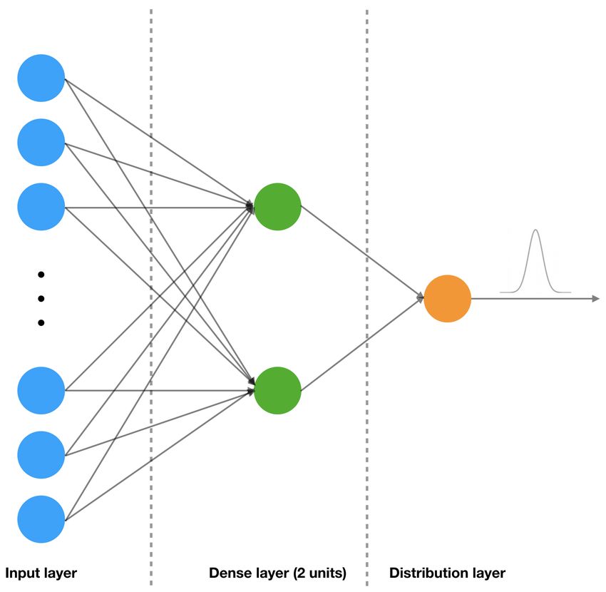
cells their density value, we can extract from each of them a The architecture of the implemented NN is schematically
certain number of points that depend on the density of the cat- represented in Figure 2. It consists of the following layers:
alogue and on the visibility function. These points represent the – Input layer that feeds the 30 values of the measured 2PCF to
galaxies of the output mock catalogue. the model;
As an illustrative example, Figure 1 shows different mea- – Dense layer2 with 2 units;
sures of the 2PCF obtained in the scale range 8 < s [h−1 Mpc] < – Distribution layer that uses the two outputs of the dense layer
50, in 30 logarithmic bins of s, and assuming the lowest and as mean and standard deviation to parameterise a Gaussian
the highest values of Ωm that have been considered in this work, distribution, which is given as output.
that are Ωm = 0.24 and Ωm = 0.38. The black and red dots
show the measures obtained from the corresponding two sets of This architecture has been chosen because it is the simplest
50 log-normal mock galaxy catalogues, while the dashed lines one we tested which is able to provide accurate cosmological
are the theoretical 2PCF models assumed to construct them. constraints. Deeper models have been tried out, but no significant
As expected, the average 2PCFs of the two sets of log-normal differences were spotted in the output predictions.
catalogues are fully consistent with the corresponding theoret-
ical predictions. Indeed, a mock log-normal catalogue charac-
terised by Ωm = Ωm,i provides a training example for the NN de- 4.2. Training and validation
scribing how galaxies would be distributed if Ωm,i was the true The training and validation sets are constructed separately, and
value. Finally, the blue and green squares show the 2PCFs of consist of 2 000 and 800 examples, respectively. Regression ma-
the real BOSS catalogue obtained by assuming Ωm = 0.24 and chine learning models work better if the range of possible out-
Ωm = 0.38, respectively, when converting galaxy redshifts into puts is well represented in the training and validation sets. We
comoving coordinates. The differences in the latter two measures construct mock catalogues with 40 different values of Ωm : 29
are caused by geometric distortions. As can be seen, neither of from Ωm = 0.24 to Ωm = 0.38 with ∆Ωm = 0.005 and 11 from
these two data sets are consistent with the corresponding 2PCF Ωm = 0.2825 to Ωm = 0.3325, also separated by ∆Ωm = 0.005.
theoretical models, that is both Ωm = 0.24 and Ωm = 0.38 ap- The latter are added to improve the density of inputs in the region
pear to be bad guesses for the real value of Ωm . As we will show
in Section 5, the NN presented in this work is not significantly 2
A layer is called dense if all its units are connected to all the units of
affected by geometric distortions. the previous layer.
Article number, page 4 of 7N. Veronesi et al.: Cosmological exploitation of Neural Networks: constraining Ωm from BOSS
the loss function means both to drive the mean values of the out-
put Gaussian distributions towards the values of the labels (i.e.
the values of Ωm corresponding to the inputs), and to reduce as
much as possible the standard deviation of those distributions.
During the training process, the interval of the labels, that
is 0.24 ≤ Ωm ≤ 0.38, has been mapped into [0, 1] through the
following linear operation:
l − 0.24
L= , (9)
0.14
where l is the original label and L is the one that belongs to the
[0, 1] interval. Once the mean, µL , and the standard deviation,
σL , of the predictions are obtained in output, we convert them
back to match the original interval of the labels. The standard
deviation is then computed as follows:
dµL dµl
= , (10)
dσL dσl
where σ is the standard deviation of µ, so that the uncertainty on
µ is given by 0.14 σL .
Fig. 2. Schematic representation of the regression model considered in 4.3. Test
this work. The input layer is represented by blue dots, the hidden dense The test set consists of 5 different 2PCF measures obtained from
layer by green dots, and the output layer by the orange dot.
log-normal mock catalogues with 16 different randomly gener-
ated values of Ωm . Therefore, we have a total of 80 measures.
that had proven to be the one where the predictions were more The Ωm predictions and uncertainties are estimated as the mean
likely, during the first attempts of the NN training. The training and standard deviation of the Gaussian distributions obtained
and validation sets consist of 50 and 20 2PCF measures for each in output (Matthies 2007; Der Kiureghian & Ditlevsen 2009;
value of Ωm , respectively. All the mock catalogues used for the Kendall & Gal 2017; Russell & Reale 2019). Our model is thus
training and validation have the same dimension of the BOSS able to associate to every point of the input space an uncertainty
2PCF measures. on the output that depends on the intrinsic scatter of the 2PCF
The loss function used for the training process is the follow- measures.
ing:
N
X
J=− log pi , (8)
i=1
where N is the number of examples and pi are the values of the
Gaussian prediction on a given example, for the true value of Ωm
of that example.
During the training process, we apply the Adam optimisation
(see Kingma & Ba 2014, for a detailed description of its func-
tioning and parameters) with the following three different steps:
– 750 epochs with η = 0.002 ,
– 150 epochs with η = 0.001 ,
– 100 epochs with η = 0.0005 ,
where η indicates the learning rate. During the three steps, the
values of the other two parameters of this optimisation algorithm
are kept fixed to β1 = 0.9 and β2 = 0.999, and the training set
was not divided into batches. Variations in the parameters of the
optimization have been performed and did not lead to signifi-
cantly different outputs.
Gradually reducing the learning rate during the training helps
the model to find the correct global minimum of the loss func-
tion (Ntampaka et al. 2019). The first epochs, having a higher
learning rate, lead the model towards the area surrounding the Fig. 3. Values of Ωm and related uncertainties predicted by our NN,
global minimum, while the last ones, having a lower learning compared with the best-fit linear model (dashed line). The best-fit slope
rate, and therefore being able to take smaller and more precise is 0.995±0.014, while the best-fit normalisation is 0.001±0.005. The er-
steps in the parameter space, have the task to lead the model to- ror bars in this plot represent the standard deviations of the distributions
wards the bottom of that minimum. In this model, minimizing for Ωm obtained as output of the NN
Article number, page 5 of 7A&A proofs: manuscript no. main
Figure 3 shows the predictions on the test set, compared to 6. Conclusions
the true values of Ωm the mocks in the test were constructed with.
As can be seen, the implemented NN is able to provide reliable In this work we investigated a supervised machine learning data
predictions when fed with measures from mock catalogues char- analysis method aimed at constraining Ωm from observed galaxy
acterised by Ωm values that were not used during the training catalogues. Specifically, we implemented a regression NN that
and validation phases. In fact, fitting this data set with a linear has been trained and validated with mock measurements of the
model: 2PCFs of BOSS galaxies. Such measures are used as a conve-
nient summary statistics of the large-scale structure of the Uni-
Ωm
pred
= α · Ωtrue verse. The goal of this work was to infer cosmological con-
m +β, (11)
straints without relying on any analytic 2PCF model to construct
we get α = 0.995 ± 0.014 and β = 0.001 ± 0.005, which are the likelihood function.
consistent with the slope and the intercept of the bisector of the To train and validate our NN, we use 2 800 2PCF examples,
quadrant. constructed with 40 different values of Ωm , in 0.24 ≤ Ωm ≤
0.38. The trained NN has been finally applied to the real 2PCF
monopole of the BOSS galaxy catalogue. We get Ωm = 0.309 ±
5. Application to BOSS data 0.008, which is in remarkable agreement with the value found
by Alam et al. (2017).
After training, validating and testing the NN, we can finally ap- This work confirms that NNs can be powerful tools also for
ply it to the real 2PCF of the BOSS galaxy catalogue. To test the cosmological inference analyses. One obvious improvement of
impact of geometric distortions caused by the assumption of a the presented work would be to consider more accurate mock
particular cosmology during the measure, we apply the NN on catalogues than the log-normal ones, for the training, validation
40 measures of the 2PCF of BOSS galaxies obtained with dif- and test phases. In particular, N-body or hydrodynamic simu-
ferent assumptions on the value of Ωm when converting from lations would be required to exploit higher-order statistics, as
observed to comoving coordinates. in particular the three-point correlation function, as features to
Figure 4 shows the results of this analysis, compared with the feed the model with. The higher the number of reliable features
Ωm constraints provided by Alam et al. (2017). The predictions is, the more accurate the predictions of the NN will be. Further-
more, multi-labeled regression models can be used to make pre-
dictions on multiple cosmological parameters at the same time.
To do that, however, bigger data sets are required, in order to
have a proper mapping of the input space, characterised by the
different values each label can have. The analysis presented in
this work should also be extended to larger scales, though in this
case more reliable mock catalogues are required not to introduce
biases in the training, in particular at the Baryon Acoustic Os-
cillations scales. Finally, a similar analysis as the one performed
in this work could be done using the density map of the cata-
logue, or directly the observed coordinates of the galaxies. This
approach would be less affected by the adopted data compression
methods considered. On the other hand, it would have a signifi-
Fig. 4. Machine learning predictions (black dots and bars) on Ωm from cantly larger computational cost for the training, validation and
the measured 2PCF of BOSS galaxies, as a function of the Ωm assumed test phases, which should be estimated with a dedicated feasibil-
in the measurements. The predictions are compared to the Ωm con- ity study. All the possible improvements described above will be
straints provided by Alam et al. (2017), here represented by the green investigated in forthcoming papers.
stripe.
of the NN have been fitted with a linear model: Acknowledgements
Ωm
pred
= α · Ωass We acknowledge the use of computational resources from
m +β, (12)
the parallel computing cluster of the Open Physics Hub
pred (https://site.unibo.it/openphysicshub/en) at the Physics and As-
where Ωm is the prediction of the regression model, while
tronomy Department in Bologna. FM and LM acknowledge the
Ωass
m is the value assumed to measure the 2PCF. The best fit- grants ASI n.I/023/12/0 and ASI n.2018-23-HH.0. LM acknowl-
values of the parameters we get are α = −0.001 ± 0.025 and
edges support from the grant PRIN-MIUR 2017 WSCC32.
β = 0.309 ± 0.008. In particular, the slope is consistent with
Software: Numpy (Harris et al. 2020); Matplotlib (Hunter
zero, that is all the Ωm predictions are consistent, within the
2007); SciPy (Virtanen et al. 2020); CosmoBolognaLib
uncertainties, independently of the value assumed in the mea-
(Marulli et al. 2016); CAMB (Lewis et al. 2000); FFTLog (Hamil-
surement. This demonstrates that the NN is indeed able to make
ton 2000); TensorFlow (Abadi et al. 2015); Keras (Chollet
robust predictions over observed data, without being biased by
et al. 2015).
geometric distortions.
Our final Ωm constraint is thus estimated from the best-fit
normalization, β, that is References
Ωm = 0.309 ± 0.008 . (13) Abadi, M., Agarwal, A., Barham, P., et al. 2015, TensorFlow: Large-Scale Ma-
chine Learning on Heterogeneous Systems, software available from tensor-
flow.org
This result is remarkably consistent with the one obtained by Aghanim, N., Akrami, Y., Ashdown, M., et al. 2018, arXiv preprint
Alam et al. (2017), which is Ωm = 0.311 ± 0.006. arXiv:1807.06209
Article number, page 6 of 7N. Veronesi et al.: Cosmological exploitation of Neural Networks: constraining Ωm from BOSS
Alam, S., Albareti, F. D., Prieto, C. A., et al. 2015, The Astrophysical Journal
Supplement Series, 219, 12
Alam, S., Ata, M., Bailey, S., et al. 2017, Monthly Notices of the Royal Astro-
nomical Society, 470, 2617
Alam, S., Ho, S., & Silvestri, A. 2016, Monthly Notices of the Royal Astronom-
ical Society, 456, 3743
Anderson, L., Aubourg, E., Bailey, S., et al. 2014, Monthly Notices of the Royal
Astronomical Society, 441, 24
Aragon-Calvo, M. A. 2019, Monthly Notices of the Royal Astronomical Society,
484, 5771
Bel, J., Marinoni, C., Granett, B., et al. 2014, Astronomy & Astrophysics, 563,
A37
Blanchard, A., Camera, S., Carbone, C., et al. 2020, Astronomy & Astrophysics,
642, A191
Chollet, F. et al. 2015, Keras
Cole, S., Percival, W. J., Peacock, J. A., et al. 2005, Monthly Notices of the Royal
Astronomical Society, 362, 505
Coles, P. & Barrow, J. D. 1987, Monthly Notices of the Royal Astronomical
Society, 228, 407
Coles, P. & Jones, B. 1991, Monthly Notices of the Royal Astronomical Society,
248, 1
Der Kiureghian, A. & Ditlevsen, O. 2009, Structural safety, 31, 105
Gil-Marín, H., Bautista, J. E., Paviot, R., et al. 2020, Monthly Notices of the
Royal Astronomical Society, 498, 2492
Goodfellow, I., Bengio, Y., & Courville, A. 2016, Deep learning (MIT press)
Gunn, J. E., Siegmund, W. A., Mannery, E. J., et al. 2006, The Astronomical
Journal, 131, 2332
Hamilton, A. J. S. 2000, Mon. Not. R. Astron. Soc., 312, 257
Harris, C. R., Millman, K. J., van der Walt, S. J., et al. 2020, Nature, 585, 357
Hassan, S., Andrianomena, S., & Doughty, C. 2020, Monthly Notices of the
Royal Astronomical Society, 494, 5761
Hawkins, E., Maddox, S., Cole, S., et al. 2003, Monthly Notices of the Royal
Astronomical Society, 346, 78
Hunter, J. D. 2007, Computing in Science and Engineering, 9, 90
Ishida, E. E. 2019, Nature Astronomy, 3, 680
Kaiser, N. 1987, Monthly Notices of the Royal Astronomical Society, 227, 1
Kendall, A. & Gal, Y. 2017, in Advances in neural information processing sys-
tems, 5574–5584
Kern, N. S., Liu, A., Parsons, A. R., Mesinger, A., & Greig, B. 2017, The Astro-
physical Journal, 848, 23
Kingma, D. P. & Ba, J. 2014, arXiv preprint arXiv:1412.6980
Landy, S. D. & Szalay, A. S. 1993, The Astrophysical Journal, 412, 64
Laureijs, R., Amiaux, J., Arduini, S., et al. 2011, arXiv preprint arXiv:1110.3193
Lewis, A., Challinor, A., & Lasenby, A. 2000, Astrophys. J., 538, 473
Lippich, M., Sánchez, A. G., Colavincenzo, M., et al. 2019, Monthly Notices of
the Royal Astronomical Society, 482, 1786
LSST Dark Energy Science Collaboration. 2012, Large Synoptic Survey Tele-
scope: Dark Energy Science Collaboration
Marulli, F., Veropalumbo, A., & Moresco, M. 2016, Astronomy and Computing,
14, 35
Matthies, H. G. 2007, in Extreme man-made and natural hazards in dynamics of
structures (Springer), 105–135
Mohammad, F., Bianchi, D., Percival, W., et al. 2018, Astronomy & Astro-
physics, 619, A17
Ntampaka, M., Eisenstein, D. J., Yuan, S., & Garrison, L. H. 2019, arXiv preprint
arXiv:1909.10527
Pan, S., Liu, M., Forero-Romero, J., et al. 2020, SCIENCE CHINA Physics,
Mechanics & Astronomy, 63, 1
Parkinson, D., Riemer-Sørensen, S., Blake, C., et al. 2012, Physical Review D,
86, 103518
Peebles, P. J. 1974, The Astrophysical Journal, 189, L51
Peebles, P. J. E. 1993, Principles of physical cosmology (Princeton university
press)
Pezzotta, A., de la Torre, S., Bel, J., et al. 2017, Astronomy & Astrophysics, 604,
A33
Ravanbakhsh, S., Oliva, J., Fromenteau, S., et al. 2016, in International Confer-
ence on Machine Learning, PMLR, 2407–2416
Reid, B., Ho, S., Padmanabhan, N., et al. 2016, Monthly Notices of the Royal
Astronomical Society, 455, 1553
Russell, R. L. & Reale, C. 2019, arXiv preprint arXiv:1910.14215
Samuel, A. L. 1959, IBM Journal of research and development, 3, 210
Totsuji, H. & Kihara, T. 1969, Publications of the Astronomical Society of Japan,
21, 221
Tsizh, M., Novosyadlyj, B., Holovatch, Y., & Libeskind, N. I. 2020, Monthly
Notices of the Royal Astronomical Society, 495, 1311
Villaescusa-Navarro, F. 2021, Bulletin of the American Physical Society
Virtanen, P., Gommers, R., Oliphant, T. E., et al. 2020, Nature methods, 17, 261
Xavier, H. S., Abdalla, F. B., & Joachimi, B. 2016, Monthly Notices of the Royal
Astronomical Society, 459, 3693
Article number, page 7 of 7You can also read