Assessing low-cost terrestrial laser scanners for deriving forest structure parameters

Preprints (www.preprints.org) | NOT PEER-REVIEWED | Posted: 30 July 2021 doi:10.20944/preprints202107.0690.v1

 Article

 Assessing low-cost terrestrial laser scanners for deriving forest
 structure parameters
 Atticus E. L. Stovall 1,2 Jeff W. Atkins 3
 1 University of Maryland, College Park, MD, USA; atticus@umd.edu
 2 Biospheric Sciences Laboratory, NASA Goddard Space Flight Center, Greenbelt, MD, USA
 3 Center for Forest Assessment and Syntheses, USDA Forest Service Southern Research Station, New Ellen-

 ton, SC, USA; jeffrey.atkins@usda.gov
 * Correspondence: atticus@umd.edu

 Abstract: The increasingly affordable price point of terrestrial laser scanners has led to a democra-
 tization of instrument availability, but the most common low-cost instruments have yet to be com-
 pared in terms of the consistency to measure forest structural attributes. Here, we compared two
 low-cost terrestrial laser scanners (TLS): the Leica BLK360 and the Faro Focus 120 3D. We evaluate
 the instruments in terms of point cloud quality, forest inventory estimates, tree-model reconstruc-
 tion, and foliage profile reconstruction. Our direct comparison of the point clouds showed reduced
 noise in filtered Leica data. Tree diameter and height were consistent across instruments (4.4% and
 1.4% error, respectively). Volumetric tree models were less consistent across instruments, with ~29%
 bias, depending on model reconstruction quality. In the process of comparing foliage profiles, we
 conducted a sensitivity analysis of factors affecting foliage profile estimates, showing a minimal
 effect from instrument maximum range (for forests less than ~50 m in height) and surprisingly little
 impact from degraded scan resolution. Filtered unstructured TLS point clouds must be artificially
 re-gridded to provide accurate foliage profiles. The factors evaluated in this comparison point to-
 wards necessary considerations for future low-cost laser scanner development and application in
 detecting forest structural parameters.

 Keywords: tls; tree; QSM; PAVD; foliage; sensor; lidar

 1. Introduction
 Since the early 2000s, terrestrial laser scanning (TLS) has matured into a robust, and
 tractable means of measuring forest structural attributes using light detection and ranging
 (LiDAR) from the ground [1]. TLS has been used to model branch architecture [2], quan-
 tify leaf angle distributions [3,4], assess habitat quality [5], estimate fuel loads [6–8], map
 forest microtopograpy [9,10], examine biodiversity gradients [11,12], and estimate forest
 biomass [13–18]. Forest biomass carbon storage and productivity and can be inferred from
 estimates of above-ground biomass [19,20]. However, uncertainties exist in the distribu-
 tion of above-ground biomass, affecting the understanding terrestrial sink/source status
 [21]. Ground based measurements of forest structure are the current basis for all area-wide
 estimates of aboveground biomass [22]. Tree diameter and height are traditionally related
 to destructive measures of dry biomass and carbon to create allometric scaling relation-
 ships that can be applied across forest plots [23–25]. Allometric relationships are difficult
 to create and as a result, tend to be low in sample size, spatially biased, and often exclude
 large trees [15,26]. An accurate and unbiased method of measuring forest structure
 through more direct ground-based measurements would constrain uncertainty in forest
 carbon storage and productivity [27,28].
 TLS offers non-destructive means of estimating above-ground biomass [14,16], forest
 structure [29,30], canopy complexity [31], and structural traits [32], but much of the re-
 search employing TLS technology has used high-end TLS units costing more than $75,000

 © 2021 by the author(s). Distributed under a Creative Commons CC BY license.

Preprints (www.preprints.org) | NOT PEER-REVIEWED | Posted: 30 July 2021 doi:10.20944/preprints202107.0690.v1

 USD--a price point directly limiting the widespread adoption of TLS methods. Until re-
 cently, high-end TLS units were the only commercially available units. A new generation
 of short-range (

Preprints (www.preprints.org) | NOT PEER-REVIEWED | Posted: 30 July 2021 doi:10.20944/preprints202107.0690.v1

 0.044 mrad; 122,000 points per second) for a total of 28.2 million pulses per scan. Time
 elapsed per scan was approximately 3 minutes.

 Table 1. Laser scanner overview of specifications and parameters used in the study.

 Faro Focus 120 3D Leica BLK 360

 Ranging Method Phase-shift Time-of-Flight

 Wavelength (nm) 905 nm 830 nm

 Laser Class Class 3R Class 1

 Beam Divergence 0.19 mrad 0.4 mrad

 Specified Ranging Accuracy ±2 mm 4 mm @ 10 m / 7 mm @ 20 m

 Resolution (this study) 1.768 (0.044°) ~1.3 mrad (0.074°)

 Max resolution 0.157 mrad (0.009°) 0.576 mrad (0.033°)

 Max Measurement Rate 976,000 per second 360,000 per second

 Max Range 120 m 60 m

 Scanning Time 1.5 min 3 min (at high)/1.5 mins (at medium)

 Temperature Operability 5°- 40°C 5 - 40° C

 Weight 5 kg 1 kg

 Full Color 70 Mpix 150 Mpix + Thermal

 Software Faro SCENE Cyclone REGISTER 360

 2.3 Scan Acquisition and Registration
 We reduced occlusion from the presence of high-density vegetation by scanning 5
 times in a diamond pattern oriented at approximately each cardinal direction to provide
 sufficient coverage and a standardized sampling scheme [13,15]. At times, an additional
 scan was required for full coverage. This scheme was followed for both scanners. To aid
 in post-processing scan registration, we placed 6-inch diameter polystyrene spheres atop
 fiberglass stakes throughout the plot. Multiple scans were digitally registered using the
 registration points, as described in the following section.
 The Faro TLS scans were registered in the Faro SCENE 5.4 software, where registra-
 tion targets were located and the point clouds aligned (plot registration error = 4.8 mm,
 sd = 4.8 mm). We removed all returns with intensity lower than 650 (maximum value =
 2100; [14]). Filtering low intensity returns reduces noise and ensures gaps are correctly
 identified for the PAVD analysis. We exported all single scan files in a gridded PTX for-
 mat. Gridded scan formats like PTX are useful for estimating vegetation area index as
 gaps are retained in the data and flagged by being shifted to the scan origin (0,0,0). The

Preprints (www.preprints.org) | NOT PEER-REVIEWED | Posted: 30 July 2021 doi:10.20944/preprints202107.0690.v1

 gaps are then easily associated with a specific azimuth or zenith angle because the PTX
 format is written according to the row and column in the scan grid. The registered point
 clouds were then filtered with a stray point filter. The stray point filter uses a moving 3 x
 3 grid cell window with a 20% retention and 1 m distance threshold. Finally, we exported
 the TLS data as a single merged ASCII file for stem modeling.
 The Leica BLK 360 scans were registered using Cyclone REGISTER 360. Registration
 targets were located within the point clouds of each individual scan (or setup as Cyclone
 REGISTER 360 refers to scans) and then classified as spherical targets within the software.
 Scans were then auto-aligned using the align cloud feature (plot registration error = 11.6
 mm, sd = 1.6). Cyclone REGISTER 360 provides the user with the option to remove am-
 biguous points, intensity overloaded points, and mixed-pixel points, though only the
 mixed-pixel points option provides the user with any control over how the filter is applied
 (i.e. low, medium and high settings). For this reason, all filters were turned off for this
 comparison. We exported the single merged, or “bundled” TLS scan in the same gridded
 PTX format as the Faro scans.

 2.4 Comparisons of TLS Measurements
 2.4.1 Point cloud quality
 With the fully aligned Faro and Leica point clouds we conducted a series of compar-
 isons. We evaluated the differences in point cloud quality and point density distribution
 with respect to height and range in the leaf-off scans. To evaluate noise in leaf-off condi-
 tions, we calculated the nearest neighbor distance between the two point clouds, high-
 lighting noise points (points detected greater than 8 cm difference from the Leica point
 clouds).
 2.4.2 Forestry and QSM Measurements
 We separated and modeled individual trees on each plot using an automated work-
 flow within the CompuTree software [33], described in detail in Stovall et al. [13,15]. The
 processing took place in four steps: ground point classification and DTM creation, stem
 identification, tree segmentation, and stem reconstruction with QSMs. The tree was auto-
 matically segmented from the point cloud using an iterative nearest neighbor approach,
 starting at the initial seed point on the stem and moving vertically while expanding in
 area with the expanding tree crown. On segmented trees, we estimated diameter at breast
 height (DBH), height, and total volume for 31 trees across the 0.1 ha plots. DBH was esti-
 mated at 1.3 m above ground using cylindrical least squares fitting as part of the Simple-
 Tree quantitative structure modeling (QSM) algorithm [34,35] within the CompuTree soft-
 ware [33]. Two DBH estimates are provided in the software: uncorrected or corrected,
 based on cylinder fits above and below the 1.3 m DBH height. We evaluated both DBH
 estimates. Tree height is also outputted from SimpleTree, as the tallest recorded point
 above ground for a segmented tree. To evaluate the total tree volume estimates from each
 TLS, we modeled the segmented tree point clouds using the SimpleTree method [35].

 2.4.3 Foliage Profiles
 PAVD distributions are derived from a simple calculation of the vertically resolved
 gap probability (Pgap). Pgap is calculated as:

 ( < ,θ)
 (θ, ) = 1 − (1)
 (θ)

 Where z is the height above ground and θ is the midpoint of the 5 degree zenith angle
 range used to aggregate the LiDAR returns. The equation essentially calculates the cumu-
 lative number of returns per unit height divided by the total number of outgoing laser
 pulses. In essence, as more vegetation is intercepted, the probability of a laser pulse es-
 caping the canopy decreases.

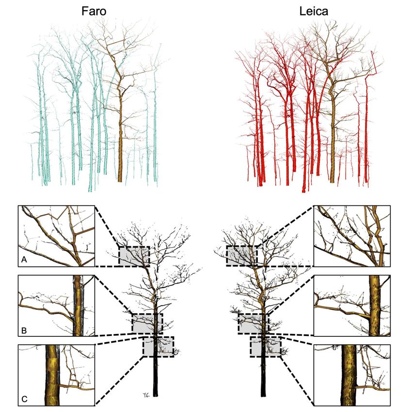
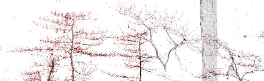
Preprints (www.preprints.org) | NOT PEER-REVIEWED | Posted: 30 July 2021 doi:10.20944/preprints202107.0690.v1

 PAVD is accurately estimated at the hinge angle - a viewing zenith angle of 57.5 de-
 grees - with Pgap. The hinge angle is used to estimate total plant area index (PAI) as this is
 the angle at which the G-Function is nearly invariable at 0.5 for all typical leaf angle dis-
 tributions [36–38]. A five-degree zenith bin between 55 and 60 degrees is used to approx-
 imate the hinge angle region. Pgap is converted to the cumulative PAI distribution with
 respect to height aboveground ( ( )) using:

 ( ) ≈ −1.1 ( (57.5)) (2)

 Estimates of ( )at the top of the canopy approximate the total PAI for a particular
 sample location. Once cumulative PAI is estimated, Pgap is calculated at 5-degree zenith
 bands from 0-60 degrees and weighted by the sin of the zenith angle to sample the upper-
 most area of the hemisphere viewable by the laser scanner. Finally, the total PAI in each 1
 m vertical bin is estimated as the 1st derivative of the ( )curve after weighting with re-
 spect to zenith angle.
 We tested the sensitivity of scanner range, resolution, and gridding on the final
 PAVD profile. For the first two tests we focused on the Faro scanner, as it had the greatest
 resolution and range in the study, making it an ideal baseline for evaluating the factors
 affecting PADV profile estimates. Scanner range was tested at 10 m intervals, excluding
 points above the range threshold of interest and then processing the resulting point cloud
 as above. Scan resolution was tested by decimating the point cloud by a factor of 10, 100,
 1,000, and 10,000. The resulting point clouds were processed as above to produce PAVD
 and PAI estimates.
 The highly filtered unstructured (not retaining the original pulse grid) Leica point
 clouds produced extreme underestimates of total PAI and PAVD, so we developed a point
 cloud gridding method useful for deriving PAI and PAVD profiles. The raw Leica data
 with xyz information is converted into zenith, azimuth, and range using a cartesian to
 spherical coordinates function. The zenith and azimuth angles can then be projected on a
 consistent artificial scan grid. In our case, the leica data was collected on a grid of ~2410
 (rows; zenith) x ~4821 (columns; azimuth). We say approximately because for a single scan
 the scan grid varies, depending on the stopping point of the laser scanner. From this we
 determined the scan resolution was ~0.075 degrees or 1.3 mrad. To ensure gaps in the scan
 data were filled we decreased the scan grid resolution by a factor of 2 to 2.6 mrad. Using
 the rasterize function in the raster package (R programming language) we created an arti-
 ficial scan grid spanning the observed zenith and azimuth range at 2.6 mrad resolution.
 For a given set of points that fall within a unique zenith and azimuth coordinate range the
 mean range value is calculated, creating a gridded set of mean TLS range observations.
 We then re-convert the gridded TLS data from spherical coordinates back to cartesian co-
 ordinates, processing using the normal PAI and PAVD processing pipeline described
 above.

 3. Results
 3.4.1 Point cloud quality
 In comparing the two scanners, there are clear differences in point cloud quality vis-
 ually as well as the distribution of observed returns. The Leica point cloud had substan-
 tially lower noise than the Faro data. Our comparison of the aligned point clouds in leaf
 off conditions highlight this issue clearly (Figure 1). The Faro data - though filtered - have
 obvious ranging errors on the edges of small objects, specifically small branches across a
 range of distances. In comparison to the Faro, a larger proportion of the returns in the
 Leica data occur at a closer distance to the scanner. The log scale distribution of returns in
 the Z-dimension show how the filtered Leica data has no returns above the canopy sur-
 face, while the Faro includes extraneous returns in the raw data. Though the Leica scanner
 is only rated to capture returns up to 60 m, we observed returns as far as 100 m in our
 comparisons of the point cloud distributions.

Preprints (www.preprints.org) | NOT PEER-REVIEWED | Posted: 30 July 2021 doi:10.20944/preprints202107.0690.v1

 Figure 1. Cross-section of Faro point cloud compared to Leica with noise points highlighted (red).
 A point was classified as noise if the distance to the Leica point cloud was greater than 8 cm point
 distances below 8 cm were assumed to be registration error.

Preprints (www.preprints.org) | NOT PEER-REVIEWED | Posted: 30 July 2021 doi:10.20944/preprints202107.0690.v1

 Figure 2. Comparison of the density of Faro and Leica returns in the [A] vertical and [B] horizontal
 dimensions.

 3.4.2 Forestry and QSM Measurements
 Tree diameter and height were in close agreement across scanners (Figure 3; Table
 2), with an RMSE of 3.8-4.0 (16-17%) for DBH, with the Faro estimating smaller values by
 ~6-10%. Tree height estimates had an RMSE of 1.1 m or 6.0% but were virtually unbiased.
 Volumetric estimates differed greatly between scanners, with the Leica having an average
 of ~0.31 or ~29% higher volume than the Faro QSMs. RMSE was ~0.6 m3 or 56%. Through
 visual inspection, we highlight key areas of the point cloud and modeling where dramatic
 differences occur (Figure 4).

 Table 2: Statistics comparing the two laser scanners. The bias estimates were relative to the Faro
 estimates. Parentheses in volume comparison show statistics excluding the largest modeled tree.

 RMSE RMSE (%) Bias Bias (%)
 DBH (cm) 3.83 16.01 1.07 4.46
 *DBH (cm) 4.03 17.33 1.32 5.69
 Height (m) 1.07 6.01 0.25 1.38
 Volume (m3) 0.61 56.33 0.31 28.97

Preprints (www.preprints.org) | NOT PEER-REVIEWED | Posted: 30 July 2021 doi:10.20944/preprints202107.0690.v1

 A 80 B 80

 ●
 ●
 60 60
 ●
 Leica Diameter (cm)

 Leica Diameter (cm)
 ●
 ●
 ● ● ●
 ●● ●● ●
 ● ● ●
 40 40
 ●● ● ●

 ●
 20 ●●●
 ● 20 ●●
 ●● ●●
 ●●●● ● ●●●●
 ● ●●● ●●
 ●●●
 ●●●
 ●● ● ●●

 0 0
 0 20 40 60 80 0 20 40 60 80
 Faro Diameter (cm) Faro Diameter (cm)

 C 40 8
 ●
 ●
 ● ●
 ●
 ●
 ●●
 30 6
 Leica Volume (m3)

 ●● ●
 Leica Height (m)

 ●
 20 ● 4
 ● ●
 ● ● ●
 ●
 ● ●
 ● ●
 10 ●● ● 2 ●
 ●●
 ●● ● ●
 ●●●●
 ●
 ●
 ●●●
 ●●
 0 ●
 0
 0 10 20 30 40 0 2 4 6 8
 3
 Faro Height (m) Faro Volume (m )

 Figure 3. Comparison of [A] uncorrected DBH, [B] corrected DBH, [C] height, and [D] total tree volume estimated from Faro and
 Leica laser scanners.

Preprints (www.preprints.org) | NOT PEER-REVIEWED | Posted: 30 July 2021 doi:10.20944/preprints202107.0690.v1

 Figure 4. [top] Overview of the resulting TLS QSMs for Faro (blue) and Leica (red) with subset tree (brown) shown in detail. The
 QSMs in comparison to the point cloud (black) show marked differences depending on instrument, with Faro point clouds having
 several inaccurate fits and Leica closely matching point cloud structure.

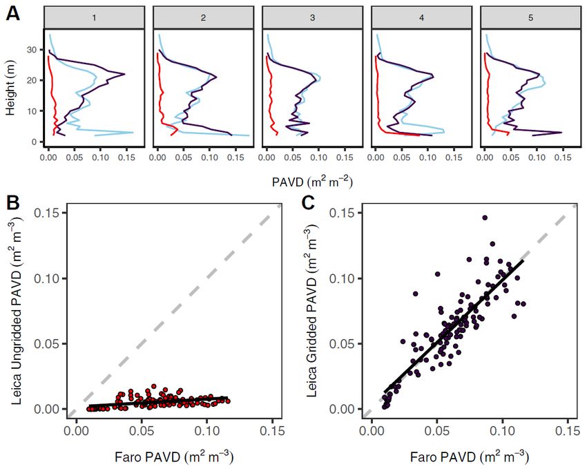
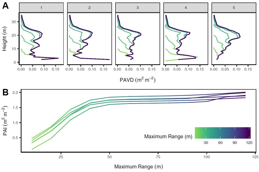
Preprints (www.preprints.org) | NOT PEER-REVIEWED | Posted: 30 July 2021 doi:10.20944/preprints202107.0690.v1

 2.4.3 Foliage Profiles
 PAVD profiles were insensitive to maximum range until ~45 m - the point where
 canopy returns nearest the scanner are lost. Below this, PAVD profiles reduce in height
 and total PAI decreases substantially (from ~2 to less than 0.5). Point cloud or laser scanner
 resolution had a minimal effect on the overall shape of the PAVD profile. Higher degra-
 dation of scanner resolution resulted in higher variability in the profile reconstructions,
 but the overall shape remained consistent. The same was true of the PAI estimates, with
 more degraded laser scans resulting in higher PAI variability. Gridding the Leica point
 cloud resulted in a closely matched PAVD profile, similar to the Faro. RMSE of the grid-
 ded PAVD profile was 0.0153 m2 m-2 or ~25% and was virtually unbiased (0.8%). In con-
 trast, the ungridded Leica data had large errors in the PAVD profile (RMSE = 100%; Bias
 = -91%).

 Figure 5. Effect of reducing maximum range on [A] vegetation profiles and [B] total Plant Area Index (PAI) at 5 scan locations
 using the Faro laser scanner. Reducing the maximum range reduces estimates of foliage profiles and PAI if the laser is unable to
 exit the canopy. Here, a ~30 m canopy requires approximately 50 m maximum range to provide unbiased estimates of PAI.

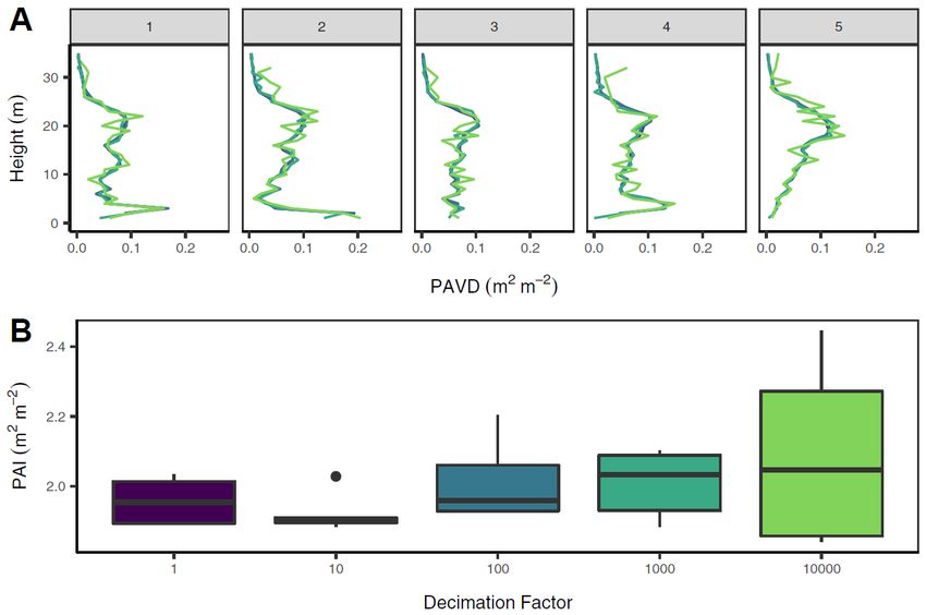
Preprints (www.preprints.org) | NOT PEER-REVIEWED | Posted: 30 July 2021 doi:10.20944/preprints202107.0690.v1

 Figure 6. Effect of point cloud resolution on [A] vegetation profiles and [B] total Plant Area Index (PAI) at the single scan level.
 Reducing point cloud resolution by decimation has little effect on the magnitude of foliage profiles and PAI, but increases
 variability across scans. Foliage profiles stayed stable up to a decimation factor of 10,000. As little as ~3000 points per scan can
 provide reliable estimates of foliage profiles, at the expense of increased variability in PAI estimates.

Preprints (www.preprints.org) | NOT PEER-REVIEWED | Posted: 30 July 2021 doi:10.20944/preprints202107.0690.v1

 Figure 7. [A] Gridded (purple) and raw filtered (red) Leica point cloud in comparison to Faro (blue) for estimates of foliage
 profiles. [B] The ungridded Leica point cloud (red) consistently underestimates PAVD. [C] Gridding the Leica data makes PAVD
 estimates comparable to the Faro data.

Preprints (www.preprints.org) | NOT PEER-REVIEWED | Posted: 30 July 2021 doi:10.20944/preprints202107.0690.v1

 4. Discussion
 We compared the ability of two low-cost terrestrial laser scanners to detect forest
 structural attributes. We assessed the point clouds from each instrument by comparing
 the return distribution and evaluating point cloud noise, clearly showing reduced noise
 in the filtered data from the Leica instrument. We further compare extracted tree-level
 diameter and height, showing consistent estimates with less than 1-5% bias. Volumetric
 estimates from QSMs were less consistent, with 29% bias, depending on model recon-
 struction quality. Finally, our sensitivity analysis of factors affecting foliage profile esti-
 mates underscored the need for scanners with appropriate range that retain all pulse in-
 formation. Surprisingly, scan resolution of extremely degraded quality produced unbi-
 ased, but variable PAI estimates. The factors evaluated in this comparison point towards
 necessary considerations for future low-cost laser scanner development and application
 in detecting forest structural parameters.

 4.1 Point Cloud Quality
 The quality of TLS point clouds is affected by a suite of instrument parameters/spec-
 ification and field conditions - all of which affect the products and estimates derived [1].
 The technology used to make ranging estimates with TLS can be phase-shift (e.g. Faro) or
 time-of-flight (e.g. Leica). Phase shift instruments are known to offer fast, high-resolution
 scans, but suffer from ranging errors for partial interceptions, such as small branches or
 leaves and edges of larger trunks (Figure 1). In contrast, time-of-flight TLS instruments
 are typically less sensitive to these edge errors, producing low-noise point clouds, but do
 not provide the same level of detail found in phase-shift TLS data. All currently available
 time-of-flight TLS have larger beam divergence than their phase-shift counterparts, con-
 sistent with the scanners in this study. Beam divergence of an instrument is the main tech-
 nical limitation for many laser scanners, since this controls the size of the laser footprint
 at distance. Larger beam divergences of time-of-flight sensors may result in an inability to
 detect small gaps in the canopy [39]. In leaf-off conditions, however, this large beam di-
 vergence is less problematic for detection of interceptions but presents issues with accu-
 rate estimates of small branch size. Here, in the winter scans, we found the Leica to pro-
 duce a much cleaner (i.e., less noise) point cloud than the Faro and, while the Leica range
 was lower, the overall quality at high distances was superior (Figure 1 and 2). This was
 particularly obvious in the presence of anomalous returns for the Faro data, where noise
 points could be found far above the forest canopy. These noise points are nearly unavoid-
 able, as they result from interference from solar radiation and inaccurate range estimates
 on the edges of objects. Filtering to the extent of removing this noise severely impacts the
 detail in point clouds, so a balance must be struck between filter parameters and presence
 of noise in these phase-shift data. In terms of point cloud quality with minimal user inter-
 vention, we conclude that the Leica provides acceptable data for single tree extraction and
 individual tree modeling, assuming appropriate quality control is implemented during
 post-processing.

 4.2 Forestry and QSM Measurements
 The fundamental basis of forest measurement lies in consistent plot-based measure-
 ments of inventory variables, such as diameter at breast height (DBH) and tree height.
 Here, we found agreement across sensors on the order of typical human error, with ~4 cm
 RMSE and 1 m for diameter and height, respectively. Since diameters were derived from
 a fully automated tree modeling process (SimpleTree) we expect even better agreement
 with algorithms optimized specifically for diameter measurement (e.g. past studies have
 sub-centimeter error [14]). Similarly, tree height estimates were derived directly from the
 derived tree-level QSMs, so point cloud approaches to height and diameter estimation
 would have likely provided much higher precision across sensors [14]. As such, we be-
 lieve measurements such as diameter and height are comparable enough for studies that

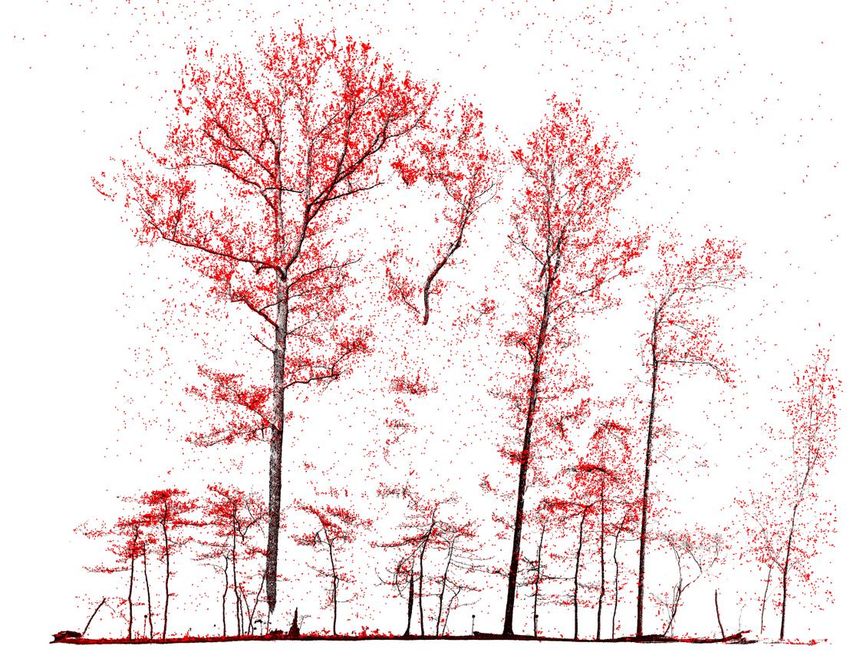
Preprints (www.preprints.org) | NOT PEER-REVIEWED | Posted: 30 July 2021 doi:10.20944/preprints202107.0690.v1

 wish to incorporate the two scanners, with the expectation that a small validation plot of
 overlapping scans is collected to provide a reference baseline for sensor agreement.
 Point cloud quality was the major factor affecting QSM-based volumetric estimates.
 Our detailed comparison of QSM fitting highlights how small errors in cylinder fits can
 result in large errors in total volume (Figure 3 and Figure 4). In general, it is clear from
 visual inspection that different representations in the small branches and noise levels di-
 rectly affect the QSM reconstruction quality. Leica estimated much higher tree volumes,
 on average, but we believe the estimates to be more accurate than Faro, since many errors
 in cylinder fits were apparent (Figure 4). The inconsistency of the two sensors with respect
 to QSM creation points to a larger issue with TLS measurements as a whole - different
 sensors can produce inconsistent data quality that ultimately propagates error and uncer-
 tainty to tree-level products [40]. In our study we ensured the scan position was virtually
 identical (within a few centimeters), but with differing scan acquisition strategies we ex-
 pect variation in upper canopy occlusion [41] will result in dramatic differences in QSM
 creation. This finding points to the need for consistent acquisition strategies that are opti-
 mized to minimize occlusion - only strategies that reduce occlusion will provide the most
 consistent estimates of tree-level volume and biomass.
 There is a clear need for objective means of evaluating point cloud and QSM quality.
 In Figure 8 we show our proposed method of providing a simple index of QSM fit quality.
 The basic method requires a simple distancing of the point cloud to the QSM cylinder
 mesh. Visualization of the residual point cloud distances (shown here as a divergent red-
 white-blue gradient) enables easy quality control of QSM creation. A statistical approach
 using this method could estimate the statistical parameters of the QSM-cloud distances,
 deriving mean and standard deviation. Here, we show how, in contrast to the Faro QSM-
 fit, the better fit from Leica data provides lower standard deviation and a mean closer to
 0. Objective methods of QSM and point cloud quality, such as these, will provide more
 consistent estimates from global-scale TLS datasets.

Preprints (www.preprints.org) | NOT PEER-REVIEWED | Posted: 30 July 2021 doi:10.20944/preprints202107.0690.v1

 Figure 8. Proposed method of evaluating QSM and point cloud quality. (top) Poor
 QSM fits are highlighted in red on the Faro point cloud. The statistics from the distri-
 bution of distances to the QSM cylinders (mean and standard deviation) can offer an
 objective method of evaluating the validity of cylinder fits across tree reconstructions.

 4.3 Foliage Profiles
 The most important instrument specifications and processing settings relevant for
 reconstructing PAVD profiles relate to range, resolution, and filtering. In our analysis, we
 found very little effect of range until the 35 m range threshold since, in a 25-30 m canopy,
 a 30-35 m range is required to exit the canopy top. As such, most TLS units have a range
 capable of measuring most canopy heights that exist globally. Of the low-cost TLS units
 evaluated here, the Faro is capable of measuring canopy structure in the tallest forest (Red-
 wood species; ~100 m; see [42] using Riegl VZ400), but the high noise with range makes
 the quality of such PAVD profiles potentially error prone. The maximum forest canopy

Preprints (www.preprints.org) | NOT PEER-REVIEWED | Posted: 30 July 2021 doi:10.20944/preprints202107.0690.v1

 height that can be measured with the Leica TLS is ~50 m, which covers a large range of
 existing forest heights, making this particular instrument broadly applicable.
 Surprisingly, PAVD profiles were minimally affected by scan resolution, with an in-
 crease in profile variability, but the broad shape and trends of the profile reconstructions
 remained consistent. The implications of these results are applicable to future low-cost
 TLS unit development. In forest stands with PAI up to ~4-5, we believe TLS units can be
 developed with lower angular resolution to reconstruct PAVD profiles. Developments
 such as this have the potential to reduce data volume and increase portability of instru-
 ments to the extent that they can become more ubiquitous in their deployment in field
 sites globally. One example of a low-cost and automated instrument specifically designed
 for forests exists (LEAF instrument, [43]. While specifications such as beam divergence
 may be a hindrance, studies of the sensitivity of parameters, as explored here, are key to
 capturing the needed technical specifications for forest-specific instruments that become
 more affordable for the scientific community.
 For the heavily filtered unstructured Leica point clouds gridding of TLS scans was
 necessary to estimate the PAVD profile. The close agreement between Leica and Faro data
 (~25% RMSE) and unbiased estimates are, in part, related to the relative insensitivity of
 the PAVD profile to scan resolution, as discussed above. However, we have uncovered a
 potential tradeoff between high quality filtered TLS data and the reconstruction of PAVD
 profiles. For example, the necessary workflow for creation of QSMs and PAVD profiles is
 specific to the desired end product. PAVD profiles may require minimum filtering of edge
 artifacts with a particular focus on clear quantification of gaps in the canopy. In contrast,
 QSM creation requires extremely clean, denoised point clouds to provide reliable results.
 As it stands, these issues remain unresolved in the TLS community and the need for a
 standardized and systematic processing workflow is necessary to ensure consistency in
 data quality as TLS is more widely adopted.

 4.4 Workflow Considerations and Recommendations
 Outside of the specific parameters tested in this study, there are marked differences
 in the field and pre-processing workflow steps between instruments, affecting the effi-
 ciency of the entire pipeline of TLS processing. Since TLS requires field-based data collec-
 tion, one major consideration in all instruments is ease of use in this setting. With several
 years of experience using the Faro instrument, the authors found field-based data collec-
 tion to be efficient and without unexpected delays. Rarely, the Faro instrument would be
 unable to operate due to temperatures outside of the safe specified range and in some
 instances instrument startup would fail; Though all situations resolved in the field and
 did not disrupt data collection. The availability of onboard touchscreen and removable
 storage space is key to ensuring data collection was successful - often revisiting a field plot
 may be impossible, so verifying data was collected successfully is essential.
 The authors found the Leica to also be efficient in field-based data collection--with
 scan acquisition times of similar magnitude to the Faro and with the added benefit of
 lighter weight, and smaller stature making moving from plot to plot easier. The Leica has
 a more restrictive temperature operating range than the Faro and does not scan below 10°
 C. A scanning campaign in central Indiana, USA had to be aborted by the authors in 2019
 simply for this reason as unseasonably cool, spring temperatures prevented scanning. The
 long-term reliability and durability of the Leica is potentially endangered by the lack of
 cover or protection for the scanning mirror and the construction of the proprietary tripod.
 While the Leica tripod is lightweight, this comes at the cost of durability as the tripod is
 not constructed to the standards required for rigorous sustained field use. Additionally,
 the Leica tripod has a specific adapter that fits the Leica, restricting the use of any other
 tripod without aftermarket modifications. The Leica also stores data internally, on a 50 gb
 solid state drive which can only be accessed via a Wi-Fi connection directly with the unit.
 Via a download management software interface, TLS scan files can then be downloaded
 in a proprietary format that must be opened with a Leica brand or related software (Cy-
 clone, Autodesk, etc.). Further Autodesk programs such as Recap Pro which can be used

Preprints (www.preprints.org) | NOT PEER-REVIEWED | Posted: 30 July 2021 doi:10.20944/preprints202107.0690.v1

 directly with the scanner in the field via an iPad wifi connection, automatically filter out
 points in a manner that the user cannot control (for which we specifically developed the
 PAVD gridding technique). While this method may be suitable for construction or archi-
 tectural work where use-cases may involve hard edges and angles, this is not adequate
 for forestry or any other ecological related work in a natural environment. The infor-
 mation loss is far too great, and the resulting data are not suitable. For example, the entire
 leaves and small branches appear to be removed from scans when this acquisition method
 is used. The only exception to this may be work quantifying microtopography [9], yet we
 advise strongly against the iPad-Autodesk/ReCap pipeline. Additionally, downloading
 files from the Leica takes several minutes per file, as does importing data into Cyclone.
 In summary, we found these two low-cost laser scanners were comparable, but key
 differences in data quality have led us to several recommendations for users of these in-
 struments. [i] The two instruments effectively and comparably estimate field inventory
 forestry measurements. We believe the simplicity of such measurements make most laser
 scanners capable of estimating these parameters and future adoption of TLS for this pur-
 pose is likely at an operational stage. [ii] QSM reconstruction is highly dependent on point
 cloud quality and thus will be directly impacted by laser scanner choice. In our case the
 higher-noise phase-shift data was problematic, resulting in less certain QSM cylinder fits,
 while low-noise time-of-flight data is best, with the expectation of potentially overesti-
 mating small branch volume due to larger beam divergence. [iii] PAVD profiles with the
 highest precision require laser scanners that retain the laser pulse grid, but artificially re-
 constructing gridded data can provide comparable PAVD profile results. While range lim-
 its on TLS instruments potentially present problems in tall forest canopies, most stationary
 laser scanners capture the range necessary to measure PAVD profiles in forest greater than
 50 m in stature. All recommendations do not point to a clear choice for the ideal laser
 scanner. Most compromises with the Leica instrument are in ease of workflow and field
 data collection, along with the lack of retained pulse grid information. The Faro instru-
 ment was efficient to use in the field and - due to the ranging technology - had far noisier
 point clouds, directly affecting the consistency of QSMs, but PAVD profiles could be re-
 constructed at a high resolution. In essence, without an available laser scanner that satis-
 fies all requirements specific to measurement of forest structure, the TLS community must
 quantify the uncertainty introduced by a particular suite of factors that directly affect
 point cloud quality and PAVD profile reconstruction; Only then can the diversity of TLS
 instruments (of all price points) be aggregated to confidently address global-scale hypoth-
 eses related to forest structure.

 Author Contributions: A.S. and J.A. conceived of the manuscript. A.S. and J.A. collected and pre-
 processed the TLS data. A.S. conducted the analyses. A.S. and J.A. wrote and edited the manuscript.

 Conflicts of Interest: The authors declare no conflict of interest.

 References

 1. Calders, K.; Adams, J.; Armston, J.; Bartholomeus, H.; Bauwens, S.; Bentley, L.P.; Chave, J.; Danson, F.M.; Demol, M.; Disney,
 M.; et al. Terrestrial Laser Scanning in Forest Ecology: Expanding the Horizon. Remote Sensing of Environment 2020, 251, 112102,
 doi:10.1016/j.rse.2020.112102.
 2. Lau, A.; Martius, C.; Bartholomeus, H.; Shenkin, A.; Jackson, T.; Malhi, Y.; Herold, M.; Bentley, L.P. Estimating Architecture-
 Based Metabolic Scaling Exponents of Tropical Trees Using Terrestrial LiDAR and 3D Modelling. Forest Ecology and
 Management 2019, 439, 132–145, doi:10.1016/j.foreco.2019.02.019.
 3. Stovall, A.E.L.; Masters, B.; Fatoyinbo, L.; Yang, X. TLSLeAF: Automatic Leaf Angle Estimates from Single-Scan Terrestrial
 Laser Scanning. New Phytologist 2021, n/a, doi:https://doi.org/10.1111/nph.17548.

Preprints (www.preprints.org) | NOT PEER-REVIEWED | Posted: 30 July 2021 doi:10.20944/preprints202107.0690.v1

 4. Vicari, M.B.; Pisek, J.; Disney, M. New Estimates of Leaf Angle Distribution from Terrestrial LiDAR: Comparison with
 Measured and Modelled Estimates from Nine Broadleaf Tree Species. Agricultural and Forest Meteorology 2019, 264, 322–333,
 doi:10.1016/j.agrformet.2018.10.021.
 5. Ashcroft, M.B.; Gollan, J.R.; Ramp, D. Creating Vegetation Density Profiles for a Diverse Range of Ecological Habitats Using
 Terrestrial Laser Scanning. METHODS IN ECOLOGY AND EVOLUTION 2014, 5, 263–272, doi:10.1111/2041-210X.12157.
 6. Loudermilk, E.L.; Hiers, J.K.; O’Brien, J.J.; Mitchell, R.J.; Singhania, A.; Fernandez, J.C.; Cropper, W.P.; Slatton, K.C. Ground-
 Based LIDAR: A Novel Approach to Quantify Fine-Scale Fuelbed Characteristics. International Journal of Wildland Fire 2009, 18,
 676–685, doi:10.1071/WF07138.
 7. Hudak, A.T.; Evans, J.S.; Stuart Smith, A.M. LiDAR Utility for Natural Resource Managers. Remote Sensing 2009, 1, 934–951,
 doi:10.3390/rs1040934.
 8. Chen, Y.; Zhu, X.; Yebra, M.; Harris, S.; Tapper, N. Development of a Predictive Model for Estimating Forest Surface Fuel Load
 in Australian Eucalypt Forests with LiDAR Data. Environmental Modelling & Software 2017, 97, 61–71,
 doi:https://doi.org/10.1016/j.envsoft.2017.07.007.
 9. Stovall, A.E.L.; Diamond, J.S.; Slesak, R.A.; McLaughlin, D.L.; Shugart, H. Quantifying Wetland Microtopography with
 Terrestrial Laser Scanning. Remote Sensing of Environment 2019, 232, 111271, doi:https://doi.org/10.1016/j.rse.2019.111271.
 10. Diamond, J.S.; McLaughlin, D.L.; Slesak, R.A.; Stovall, A. Pattern and Structure of Microtopography Implies Autogenic Origins
 in Forested Wetlands. Hydrology and Earth System Sciences 2019, 23, 5069–5088, doi:10.5194/hess-23-5069-2019.
 11. Walter, J.A.; Stovall, A.E.L.; Atkins, J.W. Vegetation Structural Complexity and Biodiversity in the Great Smoky Mountains.
 Ecosphere 2021, 12, doi:10.1002/ecs2.3390.
 12. Diamond, J.S.; McLaughlin, D.L.; Slesak, R.A.; Stovall, A. Microtopography Is a Fundamental Organizing Structure of
 Vegetation and Soil Chemistry in Black Ash Wetlands. Biogeosciences 2020, 17, 901–915, doi:10.5194/bg-17-901-2020.
 13. Stovall, A.E.L.; Shugart, H.H. Improved Biomass Calibration and Validation With Terrestrial LiDAR: Implications for Future
 LiDAR and SAR Missions. IEEE Journal of Selected Topics in Applied Earth Observations and Remote Sensing 2018, 11, 3527–3537,
 doi:10.1109/JSTARS.2018.2803110.
 14. Stovall, A.E.L.; Vorster, A.G.; Anderson, R.S.; Evangelista, P.H.; Shugart, H.H. Non-Destructive Aboveground Biomass
 Estimation of Coniferous Trees Using Terrestrial LiDAR. Remote Sensing of Environment 2017, 200, 31–42,
 doi:10.1016/j.rse.2017.08.013.
 15. Stovall, A.E.L.; Anderson-Teixeira, K.J.; Shugart, H.H. Assessing Terrestrial Laser Scanning for Developing Non-Destructive
 Biomass Allometry. Forest Ecology and Management 2018, 427, 217–229, doi:10.1016/j.foreco.2018.06.004.
 16. Calders, K.; Newnham, G.; Burt, A.; Murphy, S.; Raumonen, P.; Herold, M.; Culvenor, D.; Avitabile, V.; Disney, M.; Armston,
 J.; et al. Nondestructive Estimates of Above-Ground Biomass Using Terrestrial Laser Scanning. Methods in Ecology and Evolution
 2015, 6, 198–208, doi:10.1111/2041-210X.12301.
 17. Lau, A.; Calders, K.; Bartholomeus, H.; Martius, C.; Raumonen, P.; Herold, M.; Vicari, M.; Sukhdeo, H.; Singh, J.; Goodman,
 R.C. Tree Biomass Equations from Terrestrial LiDAR: A Case Study in Guyana. Forests 2019, 10, 527, doi:10.3390/f10060527.
 18. Momo Takoudjou, S.; Ploton, P.; Sonké, B.; Hackenberg, J.; Griffon, S.; de Coligny, F.; Kamdem, N.G.; Libalah, M.; Mofack, G.I.;
 Le Moguédec, G.; et al. Using Terrestrial Laser Scanning Data to Estimate Large Tropical Trees Biomass and Calibrate
 Allometric Models: A Comparison with Traditional Destructive Approach. Methods in Ecology and Evolution n/a-n/a,
 doi:10.1111/2041-210X.12933.
 19. Bi, H.Q.; Turner, J.; Lambert, M.J. Additive Biomass Equations for Native Eucalypt Forest Trees of Temperate Australia UR
 -://WOS:000222943100012 Http://Download.Springer.Com/Static/Pdf/888/Art%253A10.1007%252Fs00468-004-0333-
 z.Pdf?OriginUrl=http%3A%2F%2Flink.Springer.Com%2Farticle%2F10.1007%2Fs00468-004-0333-
 Z&token2=exp=1448246138~acl=%2Fstatic%2Fpdf%2F888%2Fart%25253A10.1007%25252Fs00468-004-0333-
 z.Pdf%3ForiginUrl%3Dhttp%253A%252F%252Flink.Springer.Com%252Farticle%252F10.1007%252Fs00468-004-0333-

Preprints (www.preprints.org) | NOT PEER-REVIEWED | Posted: 30 July 2021 doi:10.20944/preprints202107.0690.v1

 Z*~hmac=dc5317c0e5d26791872850f8f056e519da7d5773aaec00fa6304ff3b180b5ca4. Trees-Structure and Function 2004, 18, 467–
 479, doi:10.1007/s00468-004-0333-z.
 20. Chave, J.; Réjou-Méchain, M.; Búrquez, A.; Chidumayo, E.; Colgan, M.S.; Delitti, W.B.; Duque, A.; Eid, T.; Fearnside, P.M.;
 Goodman, R.C.; et al. Improved Allometric Models to Estimate the Aboveground Biomass of Tropical Trees. Global change
 biology 2014, 20, 3177–3190.
 21. Mitchard, E.T.A.; Feldpausch, T.R.; Brienen, R.J.W.; Lopez-Gonzalez, G.; Monteagudo, A.; Baker, T.R.; Lewis, S.L.; Lloyd, J.;
 Quesada, C.A.; Gloor, M.; et al. Markedly Divergent Estimates of Amazon Forest Carbon Density from Ground Plots and
 Satellites. Global Ecology and Biogeography 2014, 23, 935–946, doi:10.1111/geb.12168.
 22. Brown, S.; Schroeder, P.; Kern, J.S. Spatial Distribution of Biomass in Forests of the Eastern USA. Forest Ecology and Management
 1999, 123, 81–90, doi:10.1016/S0378-1127(99)00017-1.
 23. Jenkins, C.J.; Chojnacky, D.C.; Heath, L.S.; Birdsey, R.A. National-Scale Biomass Estimators for United States Tree Species. For
 Sci 2003, 49.
 24. Chojnacky, D.C.; Heath, L.S.; Jenkins, J.C. Updated Generalized Biomass Equations for North American Tree Species. Forestry
 2014, 87, 129–151.
 25. Vorster, A.G.; Evangelista, P.H.; Stovall, A.E.L.; Ex, S. Variability and Uncertainty in Forest Biomass Estimates from the Tree
 to Landscape Scale: The Role of Allometric Equations. Carbon Balance and Management 2020, 15, doi:10.1186/s13021-020-00143-
 6.
 26. Chave, J.; Condit, R.; Aguilar, S.; Hernandez, A.; Lao, S.; Perez, R. Error Propagation and Scaling for Tropical Forest Biomass
 Estimates. Philosophical Transactions of the Royal Society B: Biological Sciences 2004, 359, 409–420.
 27. Houghton, R.A.; Hall, F.; Goetz, S.J. Importance of Biomass in the Global Carbon Cycle. Journal of Geophysical Research-
 Biogeosciences 2009, 114, G00E03, doi:10.1029/2009JG000935.
 28. Land Product Validation Subgroup (Working Group on Calibration and Validation, Committee on Earth Observation
 Satellites) Aboveground Woody Biomass Product Validation Good Practices Protocol. 2021,
 doi:10.5067/DOC/CEOSWGCV/LPV/AGB.001.
 29. Fahey, R.T.; Fotis, A.T.; Woods, K.D. Quantifying Canopy Complexity and Effects on Productivity and Resilience in Late-
 Successional Hemlock–Hardwood Forests. Ecological Applications 2015, 25, 834–847, doi:10.1890/14-1012.1.
 30. Shiklomanov, A.N.; Bradley, B.A.; Dahlin, K.M.; Fox, A.M.; Gough, C.M.; Hoffman, F.M.; Middleton, E.M.; Serbin, S.P.;
 Smallman, L.; Smith, W.K. Enhancing Global Change Experiments through Integration of Remote-Sensing Techniques.
 Frontiers in Ecology and the Environment 2019, 17, 215–224, doi:10.1002/fee.2031.
 31. Atkins, J.W.; Bohrer, G.; Fahey, R.T.; Hardiman, B.S.; Morin, T.H.; Stovall, A.E.L.; Zimmerman, N.; Gough, C.M. Quantifying
 Vegetation and Canopy Structural Complexity from Terrestrial LiDAR Data Using the Forestr Package. Methods in Ecology and
 Evolution 2018, doi:10.1111/2041-210X.13061.
 32. Fahey, R.T.; Atkins, J.W.; Gough, C.M.; Hardiman, B.S.; Nave, L.E.; Tallant, J.M.; Nadehoffer, K.J.; Vogel, C.; Scheuermann,
 C.M.; Stuart‐Haëntjens, E.; et al. Defining a Spectrum of Integrative Trait‐based Vegetation Canopy Structural Types. Ecol Lett
 2019, 22, 2049–2059, doi:10.1111/ele.13388.
 33. Othmani, A.; Piboule, A.; Krebs, M.; Stolz, C.; Voon, L.L.Y. Towards Automated and Operational Forest Inventories with T-
 Lidar. In Proceedings of the 11th International Conference on LiDAR Applications for Assessing Forest Ecosystems (SilviLaser
 2011); 2011.
 34. Raumonen, P.; Kaasalainen, M.; Åkerblom, M.; Kaasalainen, S.; Kaartinen, H.; Vastaranta, M.; Holopainen, M.; Disney, M.;
 Lewis, P. Fast Automatic Precision Tree Models from Terrestrial Laser Scanner Data. Remote Sensing 2013, 5, 491–520,
 doi:10.3390/rs5020491.
 35. Hackenberg, J.; Spiecker, H.; Calders, K.; Disney, M.; Raumonen, P. SimpleTree-An Efficient Open Source Tool to Build Tree
 Models from TLS Clouds. Forests 2015, 6, 4245–4294, doi:10.3390/f6114245.
 36. MacArthur, R.H.; Horn, H.S. Foliage Profile by Vertical Measurements. Ecology 1969, 50, 802, doi:10.2307/1933693.

Preprints (www.preprints.org) | NOT PEER-REVIEWED | Posted: 30 July 2021 doi:10.20944/preprints202107.0690.v1

 37. Jupp, D.L.B.; Culvenor, D.S.; Lovell, J.L.; Newnham, G.J.; Strahler, A.H.; Woodcock, C.E. Estimating Forest LAI Profiles and
 Structural Parameters Using a Ground-Based Laser Called ‘Echidna®. Tree Physiology 2008, 29, 171–181,
 doi:10.1093/treephys/tpn022.
 38. Calders, K.; Armston, J.; Newnham, G.; Herold, M.; Goodwin, N. Implications of Sensor Configuration and Topography on
 Vertical Plant Profiles Derived from Terrestrial LiDAR. Agricultural and Forest Meteorology 2014, 194, 104–117,
 doi:10.1016/j.agrformet.2014.03.022.
 39. Newnham, G. Evaluation of Terrestrial Laser Scanners for Measuring Vegetation Structure. A Comparison of the FARO Focus
 3D 120, Leica C10, Leica HDS7000 and Riegl VZ1000. 35.
 40. Calders, K.; Disney, M.I.; Armston, J.; Burt, A.; Brede, B.; Origo, N.; Muir, J.; Nightingale, J. Evaluation of the Range Accuracy
 and the Radiometric Calibration of Multiple Terrestrial Laser Scanning Instruments for Data Interoperability. IEEE Transactions
 on Geoscience and Remote Sensing 2017, 55, 2716–2724, doi:10.1109/TGRS.2017.2652721.
 41. Wilkes, P.; Lau, A.; Disney, M.; Calders, K.; Burt, A.; Gonzalez de?Tanago, J.; Bartholomeus, H.; Brede, B.; Herold, M. Data
 Acquisition Considerations for Terrestrial Laser Scanning of Forest Plots. Remote Sensing of Environment 2017, 196, 140–153,
 doi:10.1016/j.rse.2017.04.030.
 42. Disney, M.; Burt, A.; Wilkes, P.; Armston, J.; Duncanson, L. New 3D Measurements of Large Redwood Trees for Biomass and
 Structure. Scientific Reports 2020, 10, doi:10.1038/s41598-020-73733-6.
 43. Culvenor, D.; Newnham, G.; Mellor, A.; Sims, N.; Haywood, A. Automated In-Situ Laser Scanner for Monitoring Forest Leaf
 Area Index. Sensors 2014, 14, 14994–15008, doi:10.3390/s140814994.