Field Information Modeling (FIM): Best Practices using Point Clouds - Preprints.org
←
→
Page content transcription
If your browser does not render page correctly, please read the page content below
Preprints (www.preprints.org) | NOT PEER-REVIEWED | Posted: 12 February 2021 doi:10.20944/preprints202102.0304.v1

 Technical Note

 Field Information Modeling (FIM)™: Best Practices using Point
 Clouds
 Reza Maalek 1,*

 1 Endowed Chair of Digital Engineering and Construction, Institute of Technology and Management in Con-
 struction, Karlsruhe Institute of Technology, Karlsruhe, Germany; reza.maalek@kit.edu
 * Correspondence: reza.maalek@kit.edu

 Abstract: This study presents established methods, along with new algorithmic developments, to
 automate the point cloud processing within the Field Information Modeling (FIM)™ framework.
 More specifically, given an n-D designed information model, and the point cloud’s spatial uncer-
 tainty, the problem of automatic assignment of the point clouds to their corresponding elements
 within the designed model is considered. The methods addressed two classes of field conditions,
 namely, (i) negligible construction errors; and (ii) existence of construction errors. The emphasis was
 given to describing and defining the assumptions in each method and shed light on some of their
 potentials and limitations in practical settings. Considering the shortcomings of current point cloud
 processing frameworks, three new and generic algorithms were developed to help solve the point
 cloud to model assignment in field conditions with both negligible, and existence (or speculation)
 of construction errors. The effectiveness of the new methods was demonstrated in real-world point
 clouds, acquired from construction projects, with promising results.

 Keywords: Field Information Modeling (FIM)™; point cloud to BIM; point cloud vs. BIM; n-D in-
 formation modeling; digital engineering and construction

 1. Field Information Modeling (FIM)™
 Construction project information modeling frameworks, such as building infor-
 mation modeling (BIM), heritage building information modeling (H-BIM), or bridge in-
 formation modeling (BrIM), involve modeling and integrating intelligent and semantic
 information within multi-dimensional (n-D) computer-aided design (CAD) models [1–3].
 During the design stages, the 3-dimensional (3D) digital model of a construction project
 can be created, whereby each element is classified based on attributes such as functional
 type (e.g. structural wall), elemental relationships (e.g. structural wall and floor slab con-
 nectivity and interaction), and geometric properties (e.g. shape and size) [4,5]. Further
 modeling can be carried out so as to integrate project planning and control information,
 such as work sequences and duration (e.g. 4D BIM [6]), as well as cost (e.g. 5D BIM [7]),
 enabling the project management team to directly evaluate the impact of design changes
 on the project’s schedule and cost. During construction, the designed n-D model serves as
 a detailed baseline to aid field construction work. Relevant field data must then be col-
 lected and compared to the designed model to ensure compliance. Particularly within the
 lean project delivery [8], recording fast, frequent, and reliable field data is desired to foster
 continual improvement. In the context of schedule and cost control for instance, daily
 measurement of percent planned complete, recommended as a part of the Last Planner®
 system [9], combined with frequent earned value analysis [10], require up-to-date
 knowledge of the progress of activities. Hence, Field Information Modeling (FIM)™ is
 essential to model and transform collected field data into intelligent, tangible, and seman-
 tic digital models as a means of promoting the seamless flow of information between the
 field and the digital world.
 1.1. FIM and Point Clouds

 © 2021 by the author(s). Distributed under a Creative Commons CC BY license.
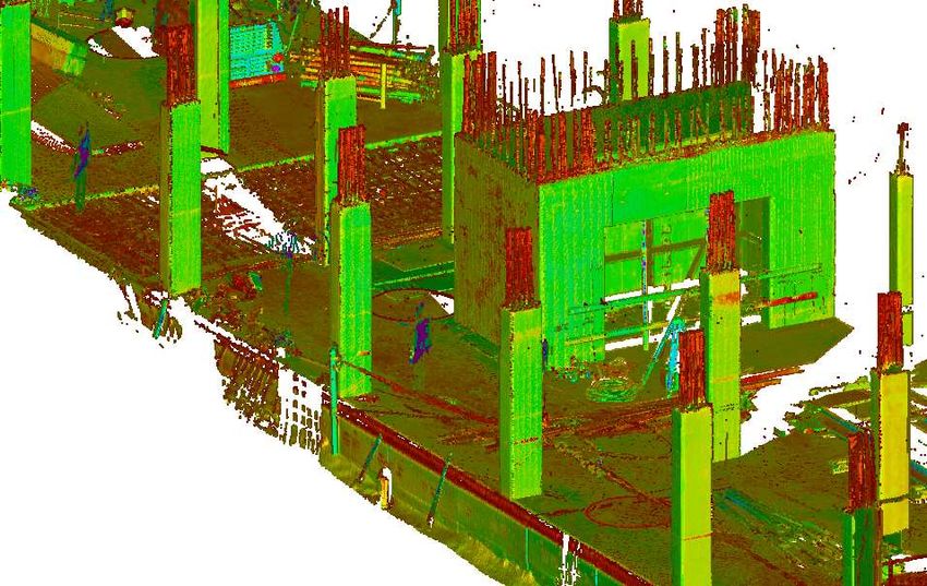
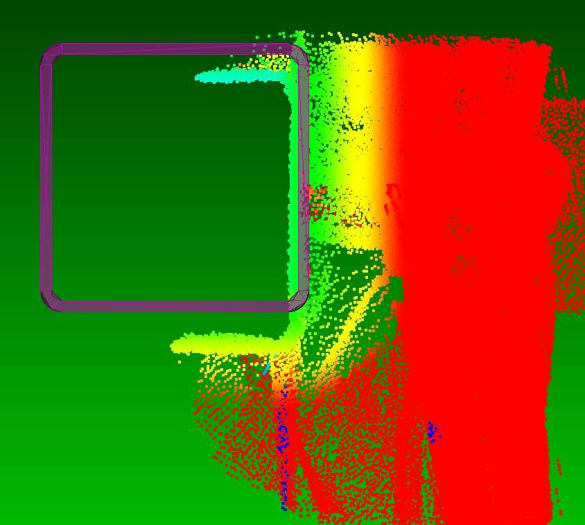
Preprints (www.preprints.org) | NOT PEER-REVIEWED | Posted: 12 February 2021 doi:10.20944/preprints202102.0304.v1

 Amongst the various types of field information that can be acquired, 3D point clouds
 provide a unique opportunity to represent surrounding real-world surfaces as discrete
 point coordinates (and in some cases with surface color or intensity information). This
 enables simultaneous control of dimensional quality (e.g. size or plumbness) as well as
 progress (e.g. percentage of complete) of field objects corresponding to work packages/ac-
 tivities [11]. Irrespective of the method used to acquire the point clouds, automated as-
 signment of points to their corresponding element in the designed n-D information model
 is an integral part of automating the FIM process.
 A typical framework to automate the assignment of points to the corresponding ele-
 ments in the designed model consists of the following steps (shown visually in Figure 1):

 3D/4D BIM/CAD/IFC ele-
 point cloud 3D/4D BIM/CAD/IFC mental classification
 (a) (b) (c)

 point cloud and model point cloud to point cloud elemental
 superimposition model comparison assignment
 (d) (e) (f)

 Figure 1. Typical framework for automatic assignment of points to the designed n-D information
 model elements: a) point cloud, b) n-D information model; c) elemental classification of the de-
 signed model; d) superimposition of the point cloud and the model; e) point cloud to model com-
 parison -in this case the color represents the distance of the points to the closest element’s surface-;
 f) result of assignment of the point cloud to their corresponding elements.

 1. Elemental classification of the design information model (Figure 1c), which is the
 process of labeling and detecting every element within the designed model based on
 criteria such as functional type and surface geometry. The surface geometry infor-
 mation related to element type already exists within the BIM, and the industry foun-
 dation class (IFC) models [4,5] and if available, can, be utilized directly. In other cases,
 particularly when only 3D CAD models exists, the STereoLithography (STL) file for-
 mat can be deployed, which approximates CAD object surfaces with triangular
 planes [12]. To further group triangular planes of the same surface together, a mesh
 segmentation process can be deployed, such as those proposed in [13–15]. The output
 of this stage is presented visually in Figure 1c, where each element is separated and
 shown with a unique color.
 2. Superimposition of the point cloud and the classified model (Figure 1d), which in-
 volves the registration of the coordinate systems of the point cloud and the model.
 To perform point cloud to model registration, at least three non-colinear point corre-
 spondences between the model and the point cloud is necessary [16]. In the presence
 of construction error, which is a reasonable assumption given the statistics related to
 rework due to poor construction [17], it is recommended to use identifiable and sig-
 nalized targets on pre-surveyed site control points to perform the registration [11,18].
 In other cases where construction errors is less prominent, iterative closest point
 (ICP) registration of the point cloud and the closest surfaces on the model can be
 performed through methods such as scan vs. BIM proposed in [12].
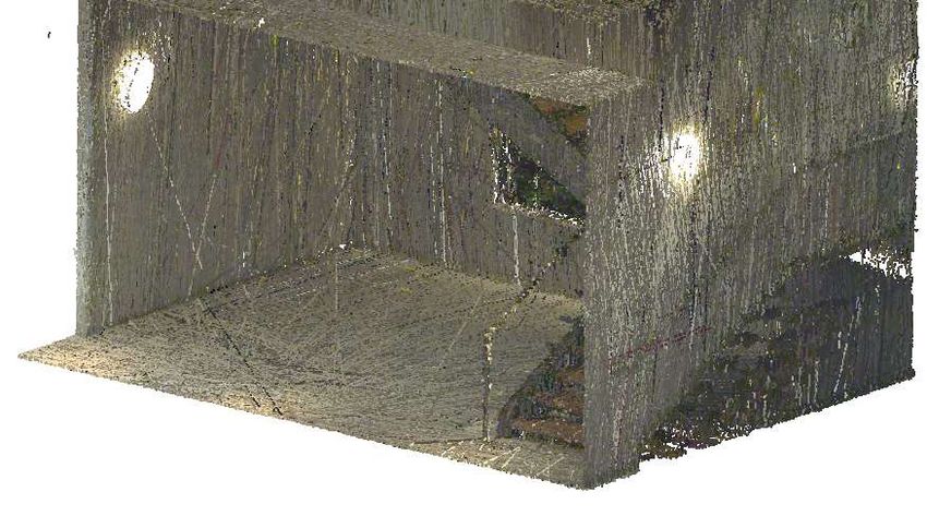
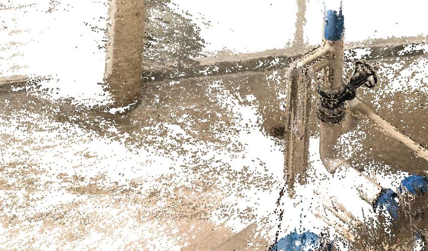
Preprints (www.preprints.org) | NOT PEER-REVIEWED | Posted: 12 February 2021 doi:10.20944/preprints202102.0304.v1 3. Point cloud to model comparison and assignment, which is used to aid with the as- signment of the point cloud to the model elements. In the case of negligible construc- tion errors, the distance of the point to the closest element can be used to determine correspondence, which is the metric used in the scan vs. BIM of [12]. A distance threshold must then be deployed to reject far points. Figure 1e shows an example of a heatmap used to visualize the distance of the points to the closest classified ele- ments. Figure 1f presents the resulting point cloud to element assignment with an arbitrarily defined distance threshold of 50mm. In other cases, where possible local construction errors exist (e.g. a set of elements are incorrectly constructed or assem- bled), the correct assignment may require to use additional information such as point neighborhood behavior [18], curvature [19], color [20] or intensity [21]. The output of stage 3 above can then be employed for progress monitoring [11,22], dimensional quality checking [11], and 3D BIM updating [23]. 1.2. Manuscript Objectives, Scope, and Structure The goal of this manuscript is to present the best practices, along with new algorith- mic developments, to automate the FIM process using point clouds, given a designed n- D information model. The scope of this study is to focus particularly on methods to solve stage 3 (and to a lesser extent stage 2) of the framework presented in Section 1.1 (Figures 1e and 1f) and using only the geometric primitives (i.e. Cartesian coordinates) of point clouds. The emphasis is given to direct frameworks, which are generalizable, robust to changes in scenery and point cloud type, and do not contain subjectively defined thresh- olds. To this end, the remainder of the manuscript is structured as follows: Section 2 describes the spatial uncertainty of point clouds and the necessity to incor- porate this spatial uncertainty within a successful point cloud processing framework. Section 3 introduces point cloud processing when construction errors can be consid- ered negligible. A new process for point cloud vs. BIM is proposed along with a demonstration of its effectiveness on real world point clouds. Section 4 reveals the basic considerations for analysis of point clouds when the im- pact of construction errors cannot be neglected. New methods for point cloud neigh- borhood definition, surface hypothesis-based classification, and surface segmenta- tion, along with demonstrated real world examples are thoroughly discussed. Section 5 summarizes the findings and provides avenues for further explorations. 2. Point Cloud Spatial Uncertainty Point clouds can be acquired through different means, such as terrestrial laser scan- ners (TLS: Figure 2a), simultaneous localization and mapping (SLAM)-based mobile sys- tems (Figure 2b), and structure-from-motion (SfM)-based photogrammetric 3D recon- struction (Figure 2c). Each point cloud collection technique has unique characteristics that impact the level of spatial uncertainty of each point measurement. A generic framework to automate point cloud processing on construction projects must, hence, incorporate the impact of point measurement uncertainties corresponding to the optical instrument [24]. Figure 2 sheds light on the importance of integrating the expected point measurement uncertainties within automated point cloud processing frameworks. Figure 2-right shows the histogram of point height, which has been shown to be an effective tool in extracting flat slab floors and ceilings from point clouds [25,26]. The points on the vicinity of the mode of the histograms represent the points of the floor (base slab). For reference, the root mean squared error (RMSE) of the points on the floor for each histogram is also shown. As illustrated, the RMSE changes from 3mm for TLS (Figure 2a-right) to 20mm for dense 3D reconstruction from smartphone cameras (Figure 2c-right). This shows that if, for in- stance, a fixed distance threshold of say 5mm is adopted to assign points around the mode of the histogram as floors, 99% of the TLS and only 32% of the smartphone 3D reconstruc- tion points will be identified as belonging to the floor. Therefore, a successful distance threshold (Figure 1f) must incorporate the expected point measurement uncertainties re- lated to a particular point cloud instrument [11,27–29].
Preprints (www.preprints.org) | NOT PEER-REVIEWED | Posted: 12 February 2021 doi:10.20944/preprints202102.0304.v1

 RMSE=~3mm

 Leica HDS6100 floor point cloud Histogram of point height
 (a)
 RMSE=~5mm

 Leica BLK2GO floor point cloud Histogram of point height
 (b)

 RMSE=~20mm

 iPhone X floor point cloud Histogram of point height
 (c)

 Figure 2. Sample point cloud (left) and histogram of point height (right) for: a) Leica HDS 6100
 TLS; b) Leica BLK2GO mobile scanner; and c) 3D reconstruction using iPhone X images.

 Given a calibrated point cloud collection instrument (assumption of modeled sys-
 tematic errors), the point measurement uncertainties in the Cartesian coordinate system
 (i.e. spatial uncertainty [28]) can be modeled through the propagation of instrumental
 measurement errors, typically approximated to the first order [30]. For instance in TLS,
 the spatial uncertainty of points must incorporate the raw instrumental measurement er-
 rors (e.g. range and angular errors; see equation 11 of [31]) along with possible scan station
 registration errors -in case of multiple scans- (see equation 5 of [11]). For each point, the
 variance propagation process provides a 3×3 covariance matrix, Σ , as measurement of
 spatial uncertainty. Closed formulations of the 3D positional uncertainty, Σ , as a function
 of instrumental measurement errors can be found in Maalek et al. [11] for TLS (Figure 1a),
 Zhengchun et al. [28] for laser radar measurement system (LRMS), Mourikis and Roume-
 liotis [32] for SLAM-based instruments (Figure 1b), and Beder and Steffen [33] for SfM-
 based techniques (Figure 1c). For each point, , the corresponding spatial uncertainty,
 Σ , can be used to construct an error ellipsoid as follows:
 ( − ) Σ ( − ) ≤ ,
 , (1)

 where , , the amplification coefficient, is considered a chi-squared probability with
 confidence, (in this study, = 97.5% is used), and degrees of freedom ( = 3 for
 3D data). Throughout the remainder of the manuscript, every point will be represented
 by its error ellipsoid using equation 1.
Preprints (www.preprints.org) | NOT PEER-REVIEWED | Posted: 12 February 2021 doi:10.20944/preprints202102.0304.v1 2.1. Assumptions of Input Parameters Before describing the methods of processing point clouds in Sections 3 and 4, it is worth outlining the basic assumptions and available input parameters, as follows: It is expected that stages 1 and 2 of the typical point cloud processing, corresponding to Figures 1a through 1d are reliably completed. This means that a point cloud from the field is acquired, the instrument by which the point cloud was collected is known, the elemental classification of the n-D designed information model is carried out, and an initial target-based registration of the point cloud and the model is performed. The point cloud instrument is assumed to be calibrated, containing no (or negligible) systematic error trends. The spatial uncertainty of each point is modeled and the error ellipsoid as per equa- tion 1 is constructed for each point. 3. Point Cloud Analysis: Case of Negligible Construction Errors This section describes the methods that can be incorporated when construction errors are considered negligible (for instance in cases of reliable pre-fabrication [34] and/or 3D printing [35] processes). This suggests that the designed n-D model and the point cloud acquired from the constructed scene must comply with little to no construction errors. Therefore, given an initial reliable point cloud to model registration, the problem of point cloud processing reduces to assigning the point to its closest element and rejecting points that are farther than a pre-defined threshold. This type of procedure was adopted for 3D reconstructed photogrammetric point clouds in Golparvar-Fard [22], and for TLS point clouds within scan vs. BIM of Bosche [12]. The two methods, however, differ in some de- tail. For the photogrammetric case, since the position and orientation of the images are estimated during the dense 3D reconstruction stage [36], Golparvar-Fard [22] proposed to perform a perspective projection of the 3D model with the same view angle at each camera position and orientation. The 3D model is now converted into a 2D image and superim- posed onto the original image to enable pixel to model assignment within each image. The image pixel is assigned to the closest 2D model pixel. The conversion of the 3D model to a 2D image possesses some merits. Firstly, since the positional uncertainties of the cameras have been already calculated during the SfM process, it can be incorporated within the assignment of each pixel to the corresponding model elements in the image. Furthermore, the assignment is performed in 2D rather than 3D, which can be faster, and if required, can allow the utilization of the many available and established image processing frame- works. The process will, however, lose efficiency when occlusions are present on site due to the loss of information with dimensionality reduction of 3D to 2D. Therefore, additional steps, such as supervised learning may be required to improve the pixel to model assign- ment in the existence of occlusions [37]. Furthermore, the process is only suited for images and cannot be generalized for point clouds acquired by other means, such as TLS. The scan vs. BIM method [12] first generates a template designed point cloud by par- allel projection of the acquired point clouds onto the closest surfaces in the designed model. The method then performs an iterative closest point (ICP) registration between the point clouds and the designed template point clouds until convergence. At each iteration only points within a distance threshold -a function of a constant distant, . , and the registration errors in the previous iteration- are used for registration and assignment. The method is attractive since it reduces the point cloud to model assignment into a template matching problem [38,39], and aims to also minimize possible target-based registration errors. The method, however, does not incorporate the impact of instrumental measure- ment errors pertaining to the point's spatial uncertainties (see Section 2). Furthermore, . was arbitrarily defined as 50mm in the study, which may not be generic for all datasets (the impact of . on the ICP registration will be demonstrated later). Finally, the ICP registration is based on point-to-point correspondences, which is known to be less accurate than point to plane registration [40,41]. Therefore, direct point cloud to plane
Preprints (www.preprints.org) | NOT PEER-REVIEWED | Posted: 12 February 2021 doi:10.20944/preprints202102.0304.v1 registration can not only improve the registration accuracy (and convergence rate), but it can also remove the necessity for generating the designed template point cloud altogether. 3.1. A New Generic Process for Point Cloud vs. Model With due consideration of the limitations of the aforementioned methods, a new ge- neric method, Algorithm 1: Point Cloud vs. Model, given the assumptions and inputs of Section 2.1, is proposed as follows: 1. Iterative improvement of the point cloud to model registration: 1.1. Assign points to corresponding planar surfaces in the model as below: 1.1.1. For each point, find the closest planar surfaces whose distance to the point is smaller than the semi-major length of the error ellipsoid (see Algorithm 5-step 2 of [11]). 1.1.2. Assign the point to the closest planar surface that intersects the error ellip- soid (ellipsoid to surface intersection is treated in Appendix A). 1.2. For each planar surface, find the inlier points of the set of points, which were assigned to the plane in step 1.1, using the method proposed in Appendix B. 1.3. Perform the closed-form point to plane registration, proposed by Khoshelham [41] to transform the inlier points onto the corresponding model planes. 1.4. Transform all points using the registration parameters of step 1.3. 1.5. Perform steps 1.1-1.4 until the points used for registration between two consec- utive iterations remain constant. 2. Assignment of non-planar points to non-planar model surfaces: 2.1. Identify the points which were not assigned to a planar surface (the remaining points after step 1). 2.2. Find the closest non-planar surface that intersects the error ellipsoid of the point (Appendix A). 2.3. For each surface in the model, perform the robust method of Appendix B to find the inlier points. 2.4. Assign the inlier points to the corresponding surface and exit the algorithm. In Algorithm 1, given a reliable registration, a point is assigned to a surface if the following two conditions are met: Its error ellipsoid intersects the surface. This is schematically shown in Figures 3a and 3b for planar and cylindrical surfaces, respectively. The intersection of ellipsoids and common surfaces such as planes, cylinders, spheres, and ellipsoids will be covered in Appendix A. The point follows the pattern of the assigned surface (an inlier point). The algorithm for detecting inlier points, given a particular model will be discussed in Appendix B. (a) (b) Figure 3. Schematic intersection of a sample ellipsoid with 3D model: a) planar surface; and b) cylindrical surface. Step 1 of Algorithm 1 involves an iterative process to improve the registration in the absence of a reliable initial target-based registration (similar to the ICP of [12]). The regis- tration process, however, only uses planar surfaces. Point to plane registration is used particularly since it is known to be accurate [40], and reliable closed-form linear solution to the point to plane registration problem already exists [41] -unlike say cylinder-based registration, which is non-linear at best [42].
Preprints (www.preprints.org) | NOT PEER-REVIEWED | Posted: 12 February 2021 doi:10.20944/preprints202102.0304.v1

 3.2. Demonstration 1: Comparison of Scan vs. BIM and Point Cloud vs. Model
 3.2.1. Experimental Setup
 Point cloud data from one rectangular concrete column with rebars on top, acquired
 from a building construction project is used (Figure 4a; data presented in [11,25]). To sim-
 ulate a model with no construction errors, the following processes are carried out:
 1. The point cloud of the sample column was subjected to a rigid body transformation
 (translation and rotation; Figure 4b).
 2. The as-built model of the rectangular column surfaces as well as the cylindrical rebars
 for the transformed point cloud was generated manually using the FARO As-built
 Modeler software [43] (Figures 4c and 4d).
 3. The original point cloud is then superimposed onto the as-built model of the trans-
 formed point cloud for comparison (Figure 4e).
 4. The proposed point cloud vs. model was compared to the scan vs. BIM method. The
 scan vs. BIM method was performed using four distance configurations with .
 changing from 50mm to 125mm in 25mm increments.

 (a) (b) (c) (d) (e)

 Figure 4. Experimental setup for demonstration 1: a) original point cloud; b) translated and ro-
 tated point cloud; c) as-built model of the transformed point cloud of Figure 4b superimposed
 onto the point cloud; d) as-built model of the transformed point cloud; and e) as-built model of the
 transformed point cloud superimposed onto the original point cloud.

 3.2.2. Results: Registration Error Comparison
 Figure 5 shows the results of the registration error in each iteration using our method
 and the four configurations of scan vs. BIM. Two main observations were made from the
 results shown in Figure 5. Firstly, scan vs. BIM appears to be considerably impacted by
 the change in . . In our data, . of 100mm and 125mm were the most optimum
 and produced almost identical registration results, whereas . of 50mm produced
 poor registration results. The second observation was that the proposed method, which is
 independent of arbitrarily defined thresholds, significantly outperformed the scan vs.
 BIM even at the most optimum distance of . = 100 . In fact, the proposed method
 after the first iteration produced better results than the converged scan vs. BIM after 30
 iterations. The proposed method converged after only four iterations and produced a final
 registration error of 0.9mm, about four times better than the best scan vs. BIM, which
 achieved 3.2mm after 30 iterations.
Preprints (www.preprints.org) | NOT PEER-REVIEWED | Posted: 12 February 2021 doi:10.20944/preprints202102.0304.v1

 Figure 5. Results of the point cloud to model registration error vs. iteration number for the pro-
 posed method, compared to scan vs. BIM [12] with . = 50 , 75 , 100 125 .

 3.2.3. Results: Quality of Point to Surface Assignment
 Given the impact of . on the registration errors, it is also important to evaluate
 the quality of point to model assignment for each method. Here, the precision, recall, ac-
 curacy and F-measure, introduced in [44] are used to define the quality of the point cloud
 to model assignment. Table 1 provides the summary of the assignment quality for each
 method. The scan vs. BIM at . of 50mm achieved comparatively poor results in both
 precision (Type I errors) and recall (Type II errors). The scan vs. BIM, however, appears
 to become more robust to Type I errors (i.e. the correct detection of points belonging to
 the surface) as the . increases from 50mm to 125mm. In fact, scan vs. BIM slightly
 outperforms our proposed method in Type I errors. Our method, however, considerably
 outperformed scan vs. BIM in Type II errors (i.e. the correct rejection of points not belong-
 ing to the surface). The latter is a consequence of the robust inlier detection (Appendix II),
 which was used within the point to surface assignment process to reject outlying points.

 Table 1. Summary of the quality of point cloud to model assignment using different methods

 Method Precision Recall Accuracy F-Measure
 Scan vs. BIM -5mm 87.9% 76.9% 69.7% 82.1%
 Scan vs BIM -75mm 98.8% 87.5% 86.6% 92.8%
 Scan vs. BIM -100 mm 100.0% 87.5% 87.5% 93.3%
 Scan vs. BIM -125 mm 100.0% 86.8% 86.8% 92.9%
 Proposed- Point Cloud vs. BIM 98.8% 99.9% 98.7% 99.3%
 * Bolded numbers represent the best value in each column

 (a)

 (b)

 Figure 6. Comparison of Type II errors during the point to model assignment: a) scan vs. BIM with
 . = 100 ; and b) proposed point cloud vs. model.

 The robustness of our proposed method to Type II errors, compared to scan vs. BIM
 with . = 100 is visually presented in Figure 6. It can be observed that many
 points of both planar and cylindrical surfaces, which are within the distance threshold of
 . = 100 , are incorrectly assigned to the surface. In our method, other than the fact
 that the distance threshold (error ellipsoid) is systematically defined based on the spatial
 uncertainty of each point, a robust surface fitting is performed to further reduce the im-
 pact of outliers and consequentially improve Type II errors.
 3.3. Constraint for Negligible Construction Error
 The aforementioned methods, e.g. scan vs. BIM, which use a distance metric to assign
 points to their corresponding elements, can only produce reliable results when the con-
 straint of negligible construction error is met. This is attributed to the fact that the presence
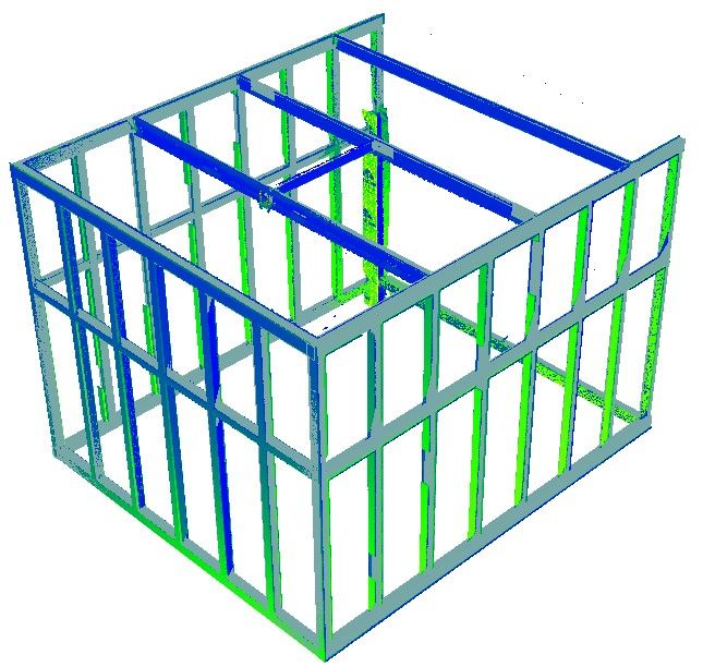
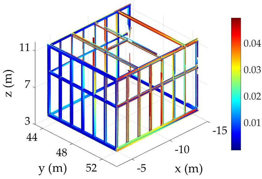
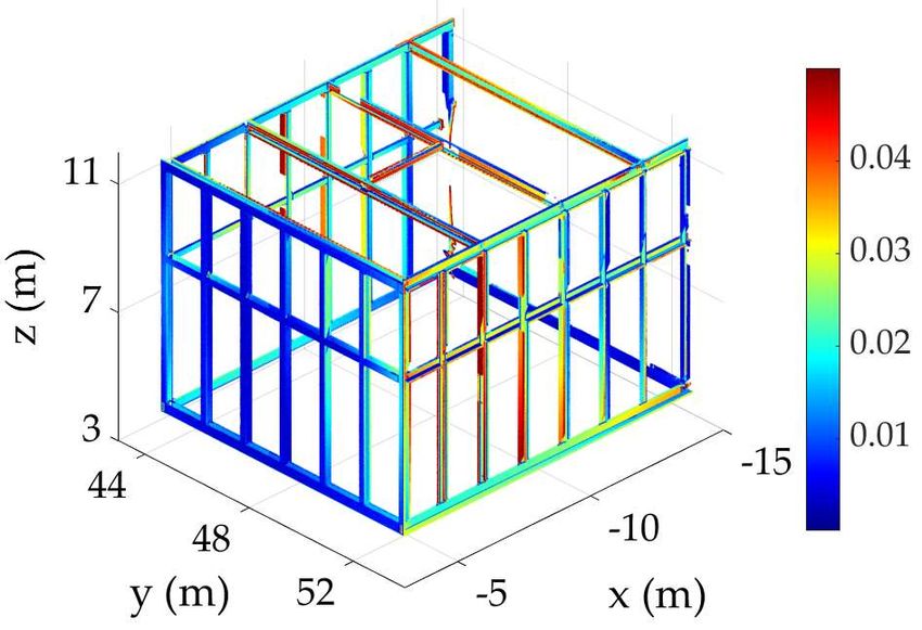
Preprints (www.preprints.org) | NOT PEER-REVIEWED | Posted: 12 February 2021 doi:10.20944/preprints202102.0304.v1

 of construction errors cannot be quantified a-priori -i.e. before the point cloud is analyzed.
 The existence of construction errors will hinder these methods in the following two ways:
 1. Distance metric: since the distance threshold is the basis for assignment or rejection
 of a point to an element, without a-priori knowledge of the construction errors, the
 threshold will be a guess at best. The impact of the subjective definition of .
 (introduced in the previous section), even for the case without construction errors,
 was thoroughly discussed in Section 3.2.
 2. Iterative registration: since the iterative ICP registration is performed on all elements,
 those elements with additional construction errors might also be used within the
 least-squares registration. Similar to any least squares adjustment in the presence of
 outliers [45], the outlying elements due to construction errors will negatively impact
 the overall registration quality. An example of this phenomena for scan vs. BIM is
 provided in Figure 7. In this example, even though the overall registration RMSE
 improved from 21mm in Figure 7a to 18mm in Figure 7b, the registration process -as
 an example- sacrificed the accuracy of the element, showed with the black arrow, to
 accommodate the element, showed in red. However, Figure 7a represents the correct
 point to model distance, and, hence, the element, shown in red, must not be allowed
 to influence the registration. It is possible to solve this problem by adopting a local
 registration and matching strategy, which will be treated in Section 4.

 (a) (b)

 Figure 7. Distance of point to 3D element model using: a) only the initial reliable target-based reg-
 istration; b) the ICP fine registration [12].

 4. Point Cloud Analysis: Existence of Construction Errors
 Construction errors is defined, here, as the possibility of a set of model elements to
 be installed and built in the field incorrectly, particularly in terms of their position, orien-
 tation and/or dimensions. The problem of damaged elements, where the geometry of the
 element is altered (e.g. a bent rectangular column) will not be considered in this manu-
 script. In the existence (or speculation) of construction errors, given an initially reliable
 registration of the point cloud and the model, each element can be treated separately and
 point cloud processing can be carried out locally (unlike the global methods described in
 Section 3). To this end, for each element, a local set of points are first isolated [27] using a
 relaxed local tolerance to account for possible construction errors (say 200mm). The as-
 signment of the isolated points to the model elements can then be treated in the following
 two ways (or in combination):
 1. Fitting the model directly to the point cloud, which aims at finding the group of
 points that match the geometry of the element. This can be accomplished by means
 of heuristic methods such as template matching [38,39], and robust least squares ad-
 justment [27,45,46].
 2. Local point cloud to model hypothesis testing, which aims at finding the points that
 locally follow the pattern of the element’s geometry.
 The difference is that the second class of methods incorporates the local geometry of each
 of the isolated points to enable point to model assignment with higher confidence. This
 additional local information may become particularly useful when assigning non-
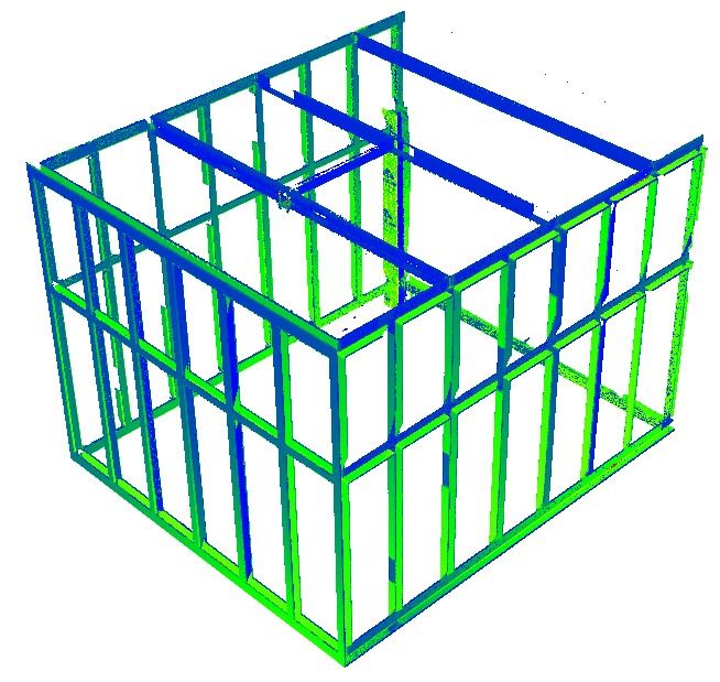
Preprints (www.preprints.org) | NOT PEER-REVIEWED | Posted: 12 February 2021 doi:10.20944/preprints202102.0304.v1

 analytical shapes in the presence of outliers. To provide some perspective, an example of
 a rectangular hollow structural section (HSS), analyzed using Verity [47] -the first ap-
 proach- is shown in Figure 8. As illustrated, due to the presence of outliers, the heuristic
 search of Verity has found a non-optimal and incorrect transformation for the HSS ele-
 ment (Figure 8b). This is particularly attributed to the fact that only a limited combination
 of points (in this case 1,000 combinations) are used, and the combination satisfying some
 decision criteria (e.g. highest consensus [48]) is selected. Additional combinations might
 improve the results, but increases the computation time without guarantee of optimality
 [49]. Local neighborhood information, such as curvature, may provide additional means
 to support the point cloud to model assignment [19]. The remainder of this section is ded-
 icated to presenting new methods to address class 2, local point cloud to model hypothesis
 testing.

 (a) (b)

 Figure 8. Results of heuristic model fitting of a hollow structural section (HSS) to contaminated
 point clouds using Verity: a) original registered model and point cloud; and b) result of the incor-
 rect model fitting.

 4.1. Local Point Cloud to Model Hypothesis Testing
 Given the geometric representation of the element in the design model, the problem
 is to find the sets of points which locally follow the element’s geometric pattern. The prob-
 lem can be solved using Algorithm 2: Hypothesis Testing as follows:
 1. Find the local neighborhood of each point (Figures 9b and 10b).
 2. For each neighborhood, estimate the best fit parameters of the element’s surface ge-
 ometry (e.g. best fit plane Figures 9c and 10c, cylinder Figure 10e, and etc.), and rec-
 ord the RMSE of the fit1, .
 3. Determine the distribution of the RMSE (Figures 9d, 10d and 10f) if the points were
 to follow the hypothesized model as follows:
 3.1. Project the points onto the best fit model (perspective projection is recommended
 for optical instruments such as perspective cameras and TLS)
 3.2. Subject the projected points to additive measurement errors (Figures 9c, 10c and
 10e) by simulating a point within the error ellipsoid of the original point to ac-
 count for the spatial uncertainty (equation 1).
 3.3. Calculate the RMSE of the best fit to the points subjected to spatial uncertainties
 3.4. Perform steps 3.1 through 3.3 times to develop the distribution of the RMSE.
 4. From step 3, record the maximum, , mean of the RMSE, , and stand-
 ard deviation of the RMSE, . , of the simulated RMSE distribution.
 5. The point belongs to the surface type if and only if the following condition is met:
 ≤ max{ | + 3 .} , (2)

 1 If an element consists of more than one surface geometry (e.g. HSS, which includes both cylindrical fillets and planar
 surfaces), perform the remaining steps on the model which achieved the lowest RMSE.
Preprints (www.preprints.org) | NOT PEER-REVIEWED | Posted: 12 February 2021 doi:10.20944/preprints202102.0304.v1 Algorithm 2 uses the surface geometry of the element, along with the spatial uncertainty of the points to simulate a probability distribution of the RMSE if the points were to follow the hypothesized geometry. The point will be designated to the geometry if and only if its RMSE complies with that of the simulated distribution. The use of Monte-Carlo simula- tion, here, enables the generation of the distribution of the RMSE, which in general form, is challenging to formulate analytically (e.g. finding the distribution of smallest eigen- value [50]). Furthermore, the distribution of the best fit parameters, such as surface nor- mal, can also be estimated during the process, which is shown to be an asset in systemat- ically determining the correct threshold for surface segmentation [31]. (a) (b) (c) (d) Figure 9. Sample of the planar hypothesis testing using Algorithm 2, applied to a neighborhood from a planar surfaces: a) point cloud; b) point cloud neighborhood of a point of desired; c) best fit plane (green), actual neighborhood points (blue), and simulated neighborhood points (magenta) - rotated such that the plane’s normal vector is parallel to the y-axis-; and d) distribution of the RMSE for the simulated planar points, where the RMSE of the actual neighborhood satisfied equa- tion 2, indicating the point follows a planar pattern. Figure 9 shows the process, described in Algorithm 2, for a neighborhood of points following a planar pattern. It can be observed from Figure 9d that the RMSE of the original point cloud neighborhood of Figure 9b, is much smaller than even the mean of the prob- ability distribution function of the RMSE of the simulated points, indicating that the point considered in Figure 9 satisfies equation 2 and follows a planar pattern. This is, in fact, not the case for the cylindrical neighborhood, shown in Figure 10. For the cylindrical neigh- borhood, if the points are projected onto the best fit plane, the RMSE of the best fit plane to the cylindrical points considerably exceeds the maximum of the probability distribution of the RMSE of the simulated planar points (Figure 10d). Alternatively, if a cylinder is fitted to the cylindrical points, the RMSE of the best fit cylinder is within the probability distribution of the RMSE of the simulated cylindrical surface, and satisfies the require- ment set in equation 2 (Figure 10f). Therefore, the point considered in Figure 9 will be classified as a plane, and the point considered in Figure 10 will be classified as a cylinder.
Preprints (www.preprints.org) | NOT PEER-REVIEWED | Posted: 12 February 2021 doi:10.20944/preprints202102.0304.v1

 (a) (b)

 (c) (d)

 (e) (f)

 Figure 10. Sample of the planar and cylindrical hypothesis testing using Algorithm 2, applied to a
 neighborhood from a cylindrical surfaces: a) point cloud; b) point cloud neighborhood of a point
 of desired; c) best fit plane (green), actual neighborhood points (blue), and simulated neighbor-
 hood points (magenta) -rotated such that the plane’s normal vector is parallel to the y-axis-; d)
 distribution of the RMSE for the simulated planar points, where the RMSE of the actual neighbor-
 hood does not satisfy equation 2, indicating the point does not follow a planar pattern; e) best fit
 cylinder (green), actual neighborhood points (blue), and simulated neighborhood points (ma-
 genta) -rotated such that the cylinder’s axis is parallel to the z-axis-; and f) distribution of the
 RMSE for the simulated cylindrical points, where the RMSE of the actual neighborhood satisfies
 equation 2, indicating the point follows a cylindrical pattern.

 Algorithm 2 is non-parametric and only requires the spatial uncertainties of the
 points from equation 1 as well as the type of geometric surface from the element’s design
 information model. Once the points are designated (classified) to the desired surface
 model (e.g. plane) using Algorithm 2, Algorithm 1 (or template matching [38]) can be uti-
 lized on only the designated points for final point to model assignment. The final consid-
 eration for Algorithm 2 is to define a reliable neighborhood around each point, and to
 determine the required number of Monte Carlo iterations, , to form a reliable distribu-
 tion of RMSE, which are discussed in the following.
 4.2. Robust Neighborhood Definition
 The neighborhood of points can be defined as fixed [25] or variable [51,52]. For the
 fixed neighborhood case, either a fixed radius around the point or a fixed number of
 neighboring points is considered. In practical settings, since the local point cloud resolu-
 tion and density vary throughout the dataset, a fixed neighborhood cannot capture the
 impact of the change in point density effectively. Variable neighborhood sizes are gener-
 ally more effective in capturing the local point density variations and consequentially bet-
 ter representing the behavior of the neighborhood of the points [51,52]. The most reliable
 methods for adaptively selecting the neighborhood of each point [51,52] utilize basic prin-
 ciples from decision and information theory [53] to find the set of points achieving the
Preprints (www.preprints.org) | NOT PEER-REVIEWED | Posted: 12 February 2021 doi:10.20944/preprints202102.0304.v1

 minimum information entropy. Theoretically the set of points with the smallest entropy
 will contain the maximum information. To this end, a range of neighborhoods are consid-
 ered, and that achieving the lowest information entropy is selected [51,52]. The two meth-
 ods presented in [51,52] differ in their definition of features used to formulate the entropy
 function with Weinmann’s formulation [51], achieving slightly better results.
 The problem of variable neighborhood can be formulated in robust statistical sense
 as finding the set of points whose determinant of the covariance matrix is minimum (MCD
 [45,54]), which is the set of points with the least outliers. Turns out that minimizing the
 determinant of the covariance matrix also minimizes the differential entropy for Gaussian
 distributions (equation 1 of [55]), which is also consistent with the principles of decision
 and information theory [53]. Hence, the optimum neighborhood can be considered as that
 achieving MCD. However, to compare the MCD as the neighborhood size increases, the
 data must be normalized, otherwise larger neighborhoods will produce greater covari-
 ance determinants. Here, the data is normalized such that the total variance, the sum of
 the eigenvalues of the covariance matrix, equals unity. The process is formulated using,
 Algorithm 3: Robust Neighborhood Definition, given starting radius (or number of
 points), , final radius, , and sampling step, , for each point as follows:
 1. Generate the sampling radius: = + . = 0: 1:
 2. For each sampling radius, , find the closest points to the point of desire within the
 spherical radius, .
 3. Calculate the eigenvalues of the covariance matrix of the set of points from step 2,
 Λ = ( , , ).
 4. Calculate the normalized MCD, , as follows:

 =∏ , (3)

 5. Select the which received the smallest .
 4.3. Demonstration 2: Evaluation of Point to Model Quality
 This sub-section involves the assessment of the effectiveness of the proposed meth-
 ods on a point cloud of a sample HSS member of Figures 9a and 10a, acquired using the
 Leica HDS6100 TLS. The sample point cloud consists of two planar surfaces and a cylin-
 drical fillet. Three experiments are described in the following, namely, robust neighbor-
 hood evaluation, impact of Monte Carlo iteration, and impact of neighborhood size.
 4.3.1. Robust Neighborhood Evaluation
 The robust neighborhood definition of Algorithm 3 is compared to the reliable vari-
 able neighborhood definition of Weinmann [51] for the data presented in Figures 9a and
 10a. The neighborhood radius was set to change from 20mm to 70mm in 1mm increments.
 The results of the defined neighborhood radius using Weinmann’s [51] and ours is visu-
 ally shown in Figure 11b and 11c, respectively. As visually illustrated, both methods pro-
 duce similar pattern of neighborhood sizes for the planar (larger neighborhoods) and cy-
 lindrical (smaller neighborhood) regions. Our method, however, appears to be more con-
 sistent with defining the neighborhood of points for the planar and cylindrical regions.
 For instance, Weinmann’s method finds a smaller neighborhood for the points of the same
 planar surface on the edges of the surface (marked in black oval), whereas ours provides
 a consistent neighborhood around the points of the same surface. Further observations
 can be made from the green ovals, which are again from the same planar surface. Overall,
 the accuracy of angle between the estimated normal and the ground truth normal vector
 was around 0.2° and 0.6°, using the proposed and Weinmann’s methods.
Preprints (www.preprints.org) | NOT PEER-REVIEWED | Posted: 12 February 2021 doi:10.20944/preprints202102.0304.v1

 (a) (b) (c)

 Figure 11. Results of the neighborhood definition: a) sample point cloud; b) Weinmann’s [51]
 method; and c) using Algorithm 3.

 4.3.2. Impact of Monte Carlo Iteration
 This experiment is designed to quantify the impact of the number of iterations, ,
 used to generate the probability distribution of the RMSE in Algorithm 2. To this end,
 Algorithm 2 in combination with Algorithm 3 was applied to the sample data with
 increasing from 25 to 1000. The quality of the planar and cylindrical classification (preci-
 sion, recall, accuracy, and F-measure) was quantified and recorded for each iteration. Fig-
 ure 12 shows the quality of the classification as the number of iterations increase. It can be
 observed that the precision, recall, accuracy, and F-measure remain relatively constant as
 the number of iterations increase from 50 to 1000. The precision, and consequentially ac-
 curacy and F-measure were, however, relatively lower with 25 iterations, compared to 50
 iterations. Therefore, 50 iterations appear to be an appropriate choice for the number of
 iterations. = 50 was also tested on the dataset shown in Figure 4a with similar results.

 Figure 12. Quality of point to model designation using Algorithm 2 vs. number of iterations

 4.3.3. Impact of Neighborhood Size
 In Section 4.3.1, it was established that the proposed neighborhood definition can
 provide accurate results, particularly to estimate the surface normal in comparison to an
 established variable neighborhood definition method. Here, the impact of fixed neighbor-
 hood sizes on the quality of the point to model designation using Algorithm 2 is evaluated.
 To this end, the neighborhood size is changed from 25mm to 75mm in 5mm increments,
 and the precision, recall, accuracy, and F-measure are recorded. Figure 13 shows the qual-
 ity of planar and cylindrical classification of Algorithm 2 ( = 50) using different fixed
 neighborhood sizes. The dashed lines show the classification quality using the robust
 neighborhood of Algorithm 3. As illustrated, the size of the neighborhood considerably
 impacts the quality of the classification. The precision appears to reduce as the neighbor-
 hood size increases. The recall, on the other hand, increases as the neighborhood size in-
 creased. Due to this counteraction between the precision and recall, the F-measure and
 accuracy peak at the neighborhood size of around 30mm. The robust neighborhood using
 Algorithm 3 provided a lower precision (indication of Type I errors), but a relatively
 higher recall (indication of Type II errors), compared to the neighborhood size of 30mm.
Preprints (www.preprints.org) | NOT PEER-REVIEWED | Posted: 12 February 2021 doi:10.20944/preprints202102.0304.v1

 In fact, the F-measure and the recall using the robust neighborhood outperformed all
 neighborhood sizes of fixed radius.
 The considerable impact of neighborhood size on the classification quality also
 demonstrates that if the data were to be isotopically scaled, the most optimum fixed neigh-
 borhood size (in this case 30mm) must also be scaled. Therefore, a fixed neighborhood
 cannot possibly provide the same point to model designation quality with models of dif-
 ferent sizes and with varying point cloud densities.

 Figure 13. Quality of point to model designation using Algorithm 2 vs. neighborhood size

 5. Concluding Remarks and Avenues for Future Exploration
 The automated analysis of point clouds, acquired from construction projects, enables
 frequent measurement and reporting of the project’s performance, which is imperative to
 promote continual improvement. To this end, this study focused on the methods to assign
 point clouds to their corresponding elements, given a reliable designed n-D model, the
 spatial uncertainty of the point clouds, and a reliable registration between the model and
 the point cloud. The methods were further sub-categorized to address field conditions
 with negligible, and existence (or speculation) of construction errors.
 In the case of negligible construction errors, a generic point cloud vs. model frame-
 work was proposed, which first performs an iterative global point to plane registration
 between the point cloud and the model. The process then assigns the points to the closest
 model elements, which intersect with the point’s error ellipsoid (representative of spatial
 uncertainty). The proposed method outperformed the popular scan vs. BIM. Scan vs. BIM
 was also found to be considerably influenced by the choice of distance threshold.
 In the existence of construction errors, it was argued that the local behavior of each
 point can provide additional information to aid with the point cloud to model assignment.
 To this end, a new generic method was proposed to designate points to classes of surface
 geometries of each element in the designed model. The method first simulates point
 clouds of the surface geometry using the spatial uncertainty of each point, and then de-
 cides if the neighborhood of the point follows the pattern of the considered class of geom-
 etry. The method is non-parametric and generic; however, it requires a process for neigh-
 borhood definition. Therefore, a new method for neighborhood definition was proposed,
 which is consistent with both robust statistics and information theory. The point cloud
 surface designation and the robust neighborhood definition was found to be promising in
 processing a real-world point cloud from an HSS member.
 Given some of the assumptions presented in this study, the following remain possi-
 ble avenues for further investigation:
 1. Automated spatial uncertainty estimation: currently, the proposed frameworks are
 predicated on the formulation of the error ellipsoid of each point a-priori. While this
 can be accomplished for most instruments, it would still be attractive to formulate
 this spatial uncertainty automatically and directly from the point cloud.
 2. Closed formulation of distribution of RMSE: Algorithm 2 involved simulating mul-
 tiple sets of points to generate the distribution of the RMSE. Formulating this RMSE
Preprints (www.preprints.org) | NOT PEER-REVIEWED | Posted: 12 February 2021 doi:10.20944/preprints202102.0304.v1

 in closed form will remove the requirement for simulating the multiple sets of points,
 which depending on the formulation, might improve computational efficiency.
 3. Point cloud assignment in the presence of damages: This study focused on errors
 during construction, including orientational, positional, and dimensional errors of a
 particular element. Automatic assignment of points to damaged elements, such as
 cracks and deformations, will be an interesting avenue for further exploration.

 Funding: The author wishes to acknowledge the support provided by the KIT Publication Fund of
 the Karlsruhe Institute of Technology in supplying the APC. This research received no additional
 external funding.
 Conflicts of Interest: The author unequivocally declares no conflict of interest.

 Appendix A: Intersection of Error Ellipsoids with Common Surfaces
 Strategies of finding intersection of ellipsoids with planes, cylinders, spheres, and
 ellipsoids are considered in the following:
 1. Ellipsoid to Plane Intersection: This problem was treated in Algorithm 5 of [11]. First,
 the error ellipsoid is converted into a sphere with radius unity through the affine
 transformation, presented in Algorithm 5-step 3 of [11]. Subject the planar surface to
 the same affine transformation. If the distance of the center of the unit sphere to the
 transformed plane is less than unity, the plane and ellipsoid have an intersection.
 2. Ellipsoid to Cylinder Intersection: This problem was treated in Algorithm 6 of [11].
 First, the cylinder and ellipsoid are rotated such that the cylinder’s axis is parallel to
 the z-axis. The problem is now reduced to checking the following two intersections
 in 2D: (i) ellipse and circle intersection in x-y plane; and (ii) ellipse and rectangle in-
 tersection in x-z (or y-z) plane. The first, ellipse and circle intersection, can be solved
 by calculating the distance of the center of the circle to the ellipse, using the method
 of Chernov [56]. If the distance is smaller than the radius of the circle (original cylin-
 der), the two curves intersect. The second, ellipse and rectangle intersection, can be
 solved using the method of Eberly [57].
 3. Ellipsoid to Ellipsoid Intersection: Wang [58] proposed an elegant algebraic condition
 for the intersection of two ellipsoids (extendable to spheres as well). It was shown
 that two ellipsoids are separated if and only if their characteristic polynomial con-
 tains exactly two distinct positive roots. This condition can be utilized to determine
 if the two ellipsoids intersect.

 Appendix B: Robust Outlier Detection
 Given a best fit model to a set of points, the following robust outlier detection algo-
 rithm, first described in Algorithm 1 and Algorithm 2 of [27] for circles, is presented:
 1. Perform the following concentration step:
 1.1. Calculate the squared residual of each point, , to the best fit model.
 1.2. Estimate the mode of , , for the intercept adjustment.
 1.3. Estimate the normalized median absolute deviation ( ; [59]) of :
 1.4. Find all points satisfying the following condition:

 ≤ . , , (B1)

 1.5. Consider the inliers as the new set of points:
 1.5.1. If the inlier points remain unchanged between two consecutive itera-
 tions, exit the concentration step and return the final set as the inliers.
 1.5.2. Else, estimate the best fit model parameters on the new points and return
 to step 1.1.
 2. Using the best fit model from the inliers of step 1, estimate the residuals, .
 3. Perform Algorithm 2 of [27] to determine all points inlier points as follows:
Preprints (www.preprints.org) | NOT PEER-REVIEWED | Posted: 12 February 2021 doi:10.20944/preprints202102.0304.v1

 3.1. Calculate the sample standard deviation of the residuals, , using the final set
 of inlier points.
 3.2. Find all points satisfying the following equation:
 | |
 ≤ . , , (B2)

 References
 1. Fu, C.; Aouad, G.; Lee, A.; Mashall-Ponting, A.; Wu, S. IFC model viewer to support nD model application. Autom. Constr.
 2006, doi:10.1016/j.autcon.2005.04.002.
 2. Ding, L.; Zhou, Y.; Akinci, B. Building Information Modeling (BIM) application framework: The process of expanding from
 3D to computable nD. Autom. Constr. 2014, doi:10.1016/j.autcon.2014.04.009.
 3. Jung, Y.; Joo, M. Building information modelling (BIM) framework for practical implementation. Autom. Constr. 2011,
 doi:10.1016/j.autcon.2010.09.010.
 4. AUTODESK Revit IFC Manual: Detailed instructions for handling IFC files;
 5. BuildingSMART IFC Standard Available online:
 https://standards.buildingsmart.org/IFC/RELEASE/IFC4/ADD1/HTML/schema/ifcgeometricmodelresource/lexical/ifcfaceb
 asedsurfacemodel.htm (accessed on Feb 6, 2021).
 6. Koo, B.; Fischer, M. Feasibility Study of 4D CAD in Commercial Construction. J. Constr. Eng. Manag. 2000,
 doi:10.1061/(asce)0733-9364(2000)126:4(251).
 7. Lee, X.S.; Tsong, C.W.; Khamidi, M.F. 5D Building Information Modelling-A Practicability Review. In Proceedings of the
 MATEC Web of Conferences; 2016.
 8. Netland, T.H. The Routledge Companion to Lean Management; Routledge: New York, NY: Routledge, 2016., 2016; ISBN
 9781315686899.
 9. Last Planner®. In Handbook for Construction Planning and Scheduling; 2014 ISBN 9781118838167.
 10. Novinsky, M.; Nesensohn, C.; Ihwas, N.; Haghsheno, S. Combined application of earned value management and last planner
 system in construction projects. In Proceedings of the IGLC 2018 - Proceedings of the 26th Annual Conference of the
 International Group for Lean Construction: Evolving Lean Construction Towards Mature Production Management Across
 Cultures and Frontiers; 2018.
 11. Maalek, R.; Lichti, D.D.; Ruwanpura, J.Y. Automatic recognition of common structural elements from point clouds for
 automated progress monitoring and dimensional quality control in reinforced concrete construction. Remote Sens. 2019, 11,
 doi:10.3390/rs11091102.
 12. Bosché, F. Automated recognition of 3D CAD model objects in laser scans and calculation of as-built dimensions for
 dimensional compliance control in construction. Adv. Eng. Informatics 2010, 24, 107–118, doi:10.1016/j.aei.2009.08.006.
 13. Yan, D.M.; Wang, W.; Liu, Y.; Yang, Z. Variational mesh segmentation via quadric surface fitting. CAD Comput. Aided Des.
 2012, doi:10.1016/j.cad.2012.04.005.
 14. Wang, J.; Yu, Z. Surface feature based mesh segmentation. In Proceedings of the Computers and Graphics (Pergamon); 2011.
 15. Wang, H.; Lu, T.; Au, O.K.C.; Tai, C.L. Spectral 3D mesh segmentation with a novel single segmentation field. Graph. Models
 2014, doi:10.1016/j.gmod.2014.04.009.
 16. Horn, B.K.P.; Hilden, H.M.; Negahdaripour, S. Closed-form solution of absolute orientation using orthonormal matrices. J.
 Opt. Soc. Am. A 1988, 5, 1127, doi:10.1364/josaa.5.001127.
 17. Hwang, B.-G.; Thomas, S.R.; Haas, C.T.; Caldas, C.H. Measuring the Impact of Rework on Construction Cost Performance. J.
 Constr. Eng. Manag. 2009, doi:10.1061/(asce)0733-9364(2009)135:3(187).
 18. Maalek, R.; Lichti, D.D.; Walker, R.; Bhavnani, A.; Ruwanpura, J.Y. Extraction of pipes and flanges from point clouds for
 automated verification of pre-fabricated modules in oil and gas refinery projects. Autom. Constr. 2019, 103,
Preprints (www.preprints.org) | NOT PEER-REVIEWED | Posted: 12 February 2021 doi:10.20944/preprints202102.0304.v1

 doi:10.1016/j.autcon.2019.03.013.
 19. Czerniawski, T.; Nahangi, M.; Haas, C.; Walbridge, S. Pipe spool recognition in cluttered point clouds using a curvature-
 based shape descriptor. Autom. Constr. 2016, doi:10.1016/j.autcon.2016.08.011.
 20. Son, H.; Kim, C.; Hwang, N.; Kim, C.; Kang, Y. Classification of major construction materials in construction environments
 using ensemble classifiers. Adv. Eng. Informatics 2014, doi:10.1016/j.aei.2013.10.001.
 21. Wang, Q.; Cheng, J.C.P.; Sohn, H. Automated Estimation of Reinforced Precast Concrete Rebar Positions Using Colored Laser
 Scan Data. Comput. Civ. Infrastruct. Eng. 2017, doi:10.1111/mice.12293.
 22. Golparvar-Fard, M.; Peña-Mora, F.; Savarese, S. Automated progress monitoring using unordered daily construction
 photographs and IFC-based building information models. J. Comput. Civ. Eng. 2015, 29, 1–19, doi:10.1061/(ASCE)CP.1943-
 5487.0000205.
 23. Rausch, C.; Haas, C. Automated shape and pose updating of building information model elements from 3D point clouds.
 Autom. Constr. 2021, 124, 103561, doi:10.1016/j.autcon.2021.103561.
 24. Rebolj, D.; Pučko, Z.; Babič, N.Č.; Bizjak, M.; Mongus, D. Point cloud quality requirements for Scan-vs-BIM based automated
 construction progress monitoring. Autom. Constr. 2017, 84, 323–334, doi:10.1016/j.autcon.2017.09.021.
 25. Maalek, R.; Lichti, D.D.; Ruwanpura, J.Y. Robust segmentation of planar and linear features of terrestrial laser scanner point
 clouds acquired from construction sites. Sensors (Switzerland) 2018, 18, doi:10.3390/s18030819.
 26. Macher, H.; Landes, T.; Grussenmeyer, P. From point clouds to building information models: 3D semi-automatic
 reconstruction of indoors of existing buildings. Appl. Sci. 2017, doi:10.3390/app7101030.
 27. Maalek, R.; Lichti, D.D.; Walker, R.; Bhavnani, A.; Ruwanpura, J.Y. Extraction of pipes and flanges from point clouds for
 automated verification of pre-fabricated modules in oil and gas refinery projects. Autom. Constr. 2019, 103, 150–167,
 doi:10.1016/j.autcon.2019.03.013.
 28. Du, Z.; Wu, Z.; Yang, J. Point cloud uncertainty analysis for laser radar measurement system based on error ellipsoid model.
 Opt. Lasers Eng. 2016, doi:10.1016/j.optlaseng.2015.11.010.
 29. Du, Z.; Wu, Z.; Yang, J. Error ellipsoid analysis for the diameter measurement of cylindroid components using a laser radar
 measurement system. Sensors (Switzerland) 2016, doi:10.3390/s16050714.
 30. Ku, H.H. Notes on the use of propagation of error formulas. J. Res. Natl. Bur. Stand. Sect. C Eng. Instrum. 1966,
 doi:10.6028/jres.070c.025.
 31. Maalek, R.; Lichti, D.D.; Ruwanpura, J.Y. Robust segmentation of planar and linear features of terrestrial laser scanner point
 clouds acquired from construction sites. Sensors (Switzerland) 2018, 18, doi:10.3390/s18030819.
 32. Mourikis, A.I.; Roumeliotis, S.I. Analysis of positioning uncertainty in Simultaneous Localization and Mapping (SLAM). In
 Proceedings of the 2004 IEEE/RSJ International Conference on Intelligent Robots and Systems (IROS); 2004.
 33. Beder, C.; Steffen, R. Determining an initial image pair for fixing the scale of a 3D reconstruction from an image sequence.
 Lect. Notes Comput. Sci. (including Subser. Lect. Notes Artif. Intell. Lect. Notes Bioinformatics) 2006, 4174 LNCS, 657–666,
 doi:10.1007/11861898_66.
 34. GOLDBECK GmbH Available online: https://www.goldbeck.de/startseite/ (accessed on Dec 11, 2020).
 35. Tay, Y.W.D.; Panda, B.; Paul, S.C.; Noor Mohamed, N.A.; Tan, M.J.; Leong, K.F. 3D printing trends in building and
 construction industry: a review. Virtual Phys. Prototyp. 2017.
 36. Schönberger, J.L. Robust Methods for Accurate and Efficient 3D Modeling from Unstructured Imagery. 2018, 277.
 37. Han, K.K.; Golparvar-Fard, M. Potential of big visual data and building information modeling for construction performance
 analytics: An exploratory study. Autom. Constr. 2017, 73, 184–198, doi:10.1016/j.autcon.2016.11.004.
 38. Vock, R.; Dieckmann, A.; Ochmann, S.; Klein, R. Fast template matching and pose estimation in 3D point clouds. Comput.
 Graph. 2019, doi:10.1016/j.cag.2018.12.007.
 39. Brunelli, R. Template Matching Techniques in Computer Vision; John Wiley & Sons, Ltd: Chichester, UK, 2009; ISBN
You can also read