Association between NO 2 concentrations and spatial configuration: a study of the impacts of COVID-19 lockdowns in 54 US cities
←
→
Page content transcription
If your browser does not render page correctly, please read the page content below
LETTER • OPEN ACCESS

Association between NO2 concentrations and spatial configuration: a
study of the impacts of COVID-19 lockdowns in 54 US cities
To cite this article: Man Sing Wong et al 2021 Environ. Res. Lett. 16 054064

View the article online for updates and enhancements.

                               This content was downloaded from IP address 73.36.175.12 on 29/05/2021 at 02:34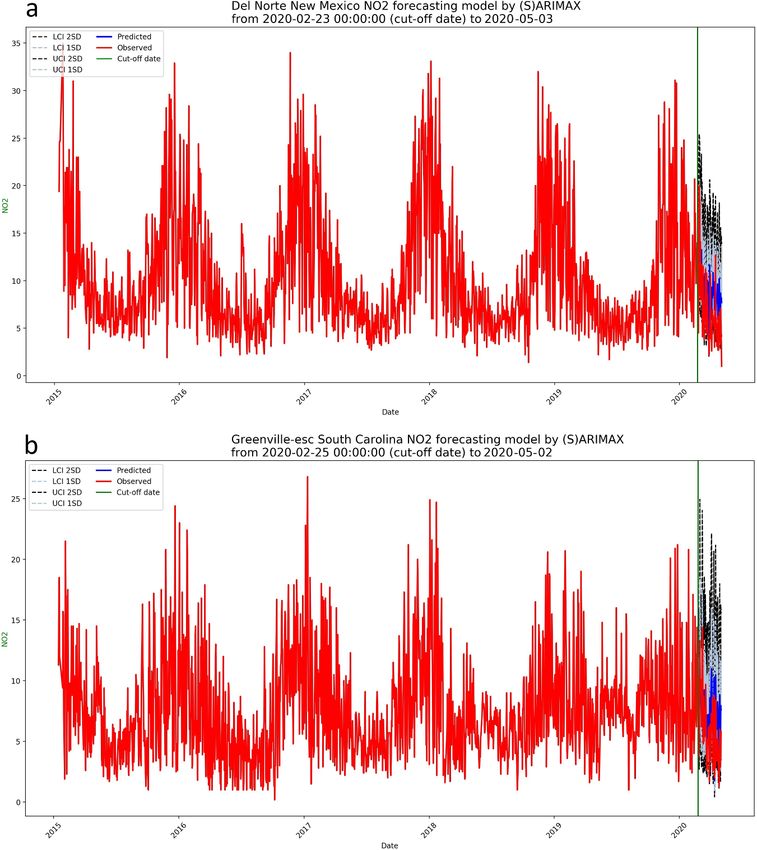
Environ. Res. Lett. 16 (2021) 054064 https://doi.org/10.1088/1748-9326/abf396
LETTER
Association between NO2 concentrations and spatial
OPEN ACCESS
configuration: a study of the impacts of COVID-19 lockdowns in
RECEIVED
6 December 2020 54 US cities
REVISED
23 March 2021 Man Sing Wong1,2, Rui Zhu1,3,∗, Coco Yin Tung Kwok1, Mei-Po Kwan4, Paolo Santi5,6, Chun Ho Liu7,
ACCEPTED FOR PUBLICATION Kai Qin8, Kwon Ho Lee9, Joon Heo10, Hon Li1 and Carlo Ratti5
30 March 2021
1
Department of Land Surveying and Geo-Informatics, The Hong Kong Polytechnic University, Kowloon, Hong Kong Special
PUBLISHED
11 May 2021 Administrative Region of China, People’s Republic of China
2
Research Institute for Sustainable Urban Development, The Hong Kong Polytechnic University, Kowloon, Hong Kong Special
Administrative Region of China, People’s Republic of China
Original Content from 3
Senseable City Laboratory, Future Urban Mobility, Singapore-MIT Alliance for Research and Technology, 1 Create Way, 09-02 Create
this work may be used
under the terms of the Tower, 138062, Singapore
4
Creative Commons Institute of Space and Earth Information Science, The Chinese University of Hong Kong, Hong Kong Special Administrative Region
Attribution 4.0 licence. of China, People’s Republic of China
5
Any further distribution Senseable City Laboratory, Department of Urban Studies and Planning, Massachusetts Institute of Technology, Cambridge, MA 02139,
of this work must United States of America
maintain attribution to 6
Istituto di Informatica e Telematica del CNR, 56124 Pisa, Italy
the author(s) and the title 7
of the work, journal Department of Mechanical Engineering, The University of Hong Kong, Hong Kong Special Administrative Region of China,
citation and DOI. People’s Republic of China
8
School of Environment Science and Spatial Informatics, China University of Mining and Technology, Xuzhou,
People’s Republic of China
9
Department of Atmospheric & Environmental Sciences, Gangneung-Wonju National University, Gangneung, Republic of Korea
10
Department of Civil and Environmental Engineering, Yonsei University, Seoul, Republic of Korea
∗
Author to whom any correspondence should be addressed.
E-mail: felix.zhu@polyu.edu.hk
Keywords: NO2 , air quality, COVID-19, lockdowns, urban mobility
Abstract
The massive lockdown of global cities during the COVID-19 pandemic is substantially improving
the atmospheric environment, which for the first time, urban mobility is virtually reduced to zero,
and it is then possible to establish a baseline for air quality. By comparing these values with
pre-COVID-19 data, it is possible to infer the likely effect of urban mobility and spatial
configuration on the air quality. In the present study, a time-series prediction model is enhanced to
estimate the nationwide NO2 concentrations before and during the lockdown measures in the
United States, and 54 cities are included in the study. The prediction generates a notable NO2
difference between the observations if the lockdown is not considered, and the changes in urban
mobility can explain the difference. It is found that the changes in urban mobility associated with
various road textures have a significant impact on NO2 dispersion in different types of climates.
1. Introduction measures are taken since March 2020 (Kucharski et al
2020). Due to the global lockdown, the coronavirus
In December 2019, the pandemic outbreak of severe disease 2019 (COVID-19) has undermined world-
acute respiratory syndrome coronavirus 2 (SARS- wide economies and triggered a global crisis due to
CoV-2) emerged in Wuhan, China, after which more great loss in the socioeconomic domain described by
than 10 million cases are confirmed and 500 000 the United Nations (UNnews 2020). It was predicted
deaths are resulted by 1 July 2020, and the pan- that global trade will decline by 13%–32% and the
demic also spread in over 250 countries in the annual global gross product is projected to decline
world. Despite the progressive increase in the num- by 24% (CRS 2020). Additionally, a strict lockdown
ber of confirmed cases every day, the situation has in China reduced global GDP by 3.5% and Chinese
become relatively stable in some countries after the GDP by 21% (Guan et al 2020). Notwithstanding, the
massive lockdown is adopted and strict travel control socioeconomy is chronically and devastatingly hit by
© 2021 The Author(s). Published by IOP Publishing Ltd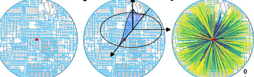
Environ. Res. Lett. 16 (2021) 054064                                                                   M S Wong et al

the disease, and the environment has responded to          and fuel decomposition, as well as the vehicle speed
the pandemic instantly (Fan et al 2020). The level of      and fleet composition (Tang et al 2019). Nevertheless,
nitrogen dioxide (NO2 ) is substantially reduced in the    it is reckoned that the improved air quality is mainly
wake of COVID-19 (Mahato et al 2019). In Central           a result of the favourable meteorological conditions
China, NO2 emission is decreased by 30% on a year-         rather than the minimized anthropogenic activities
after-year basis during the Lunar New Year compared        because the pollutant diffusivity was an important
with the period from 2005-2019 (Earth Observat-            factor closely related to meteorology (Wang et al
ory 2020). The reduction of air pollution includ-          2020).
ing NO2 is first identified appeared in Wuhan, and              Another factor that contributes to NO2 emission
such phenomena are found in more and more cities           is traffic characteristics. By investigating the correla-
and countries, and eventually it becomes a worldwide       tion between NO2 and its emission factor, research-
phenomenon (Venter et al 2020). Among 31 major             ers speculated that the deviation of the contributing
cities in the world, a significant decline in NO2 has      factors NO2 emission resulted from the variability of
been observed in almost two-thirds of the study area       the local road condition, the traffic pattern and the
after the lockdown, including New York, Rome and           fleet composition (Chan et al 2004, Liu et al 2012).
Paris, implying that the transportation and anthro-        The road 300 km or above in length was featured by
pogenic activities in the cities mentioned above were      higher NO2 concentration as shown by a study con-
massively lessened (Shrestha et al 2020). Epidemiolo-      ducted in the Netherland (Velders et al 2009), and
gical evidence suggested that the high incidence of        the study result is consistent with another finding
respiratory disease and many death tolls should be         that a higher NO2 exposure was associated with the
attributed to the deteriorated air quality (Brauer et al   road length variability in Shanghai (Meng et al 2015).
2010). For example, approximately 4.6 million indi-        Moreover, the spatial distribution and the local vari-
viduals died from the disease annually due to the low      ability of NO2 concentration (Wang et al 2020) are
air quality, as reported by the World Trade Organisa-      analytically explored, and the results show that the
tion (Cohen et al 2017), and the lung tissue can be        local variation was mostly driven by regional differ-
damaged by prolonged exposure to NO2 , which is one        ences between the ten most urbanized areas in the
of the contributors to the morbidity of asthma and         United States, which was consistent with the basic
lung cancer (Greenberg et al 2016, Khaniabadi et al        conditions of these urban regions, that is, comparat-
2017). Thus, it is of great significance to the enhance-   ively denser traffic and frequent anthropogenic emis-
ment of the atmospheric environment by grasping the        sion. Therefore, different spatio-temporal locations
evolutionary patterns of NO2 and its causal factors        and the traffic characteristics have a significant influ-
appropriately (He et al 2020).                             ence on the level of NO2 , even though some of the
     Road traffic can be regarded as the major con-        emission features result from specific industrial activ-
tributor to NO2 (Palmgren et al 2007, Keuken et al         ities. In the US metropolitan cities, the local NO2 con-
2009, Mohegh et al 2020). The rise of NO2 concen-          centrations can be improved by reducing the road
tration might cause a certain type of diesel particu-      traffic even if there is a variability of estimation error
late produced by heavy vehicles such as buses, whereas     in NO2 . Therefore, no effective prediction model
nitrogen is produced by the gasoline-fuelled passen-       has been developed for national NO2 concentration
ger cars, particularly sensitive to long-range transport   yet (Lee et al 2019).
decomposition (Carslaw et al 2005, Heeb et al 2008).            As a reliable and accurate method for math-
According to an observation of the vehicle emis-           ematical modelling, auto-regressive integrated mov-
sion factors, it is found that the decreasing trend of     ing average (ARIMA) has been widely applied to
NO2 emission is the smallest and insignificant among       short-term time-series trend analysis and its frequent
other pollutants throughout the 12 years study period      application in the prediction from multiple perspect-
in Switzerland (Hueglin et al 2006), which suggests        ives. For instance, it was adopted in the study try-
that the road traffic emission ratio in NO2 increased      ing to make an accurate forecast of wind speed at
during this period. A similar outcome means that           wind power plants and ensure the overall stability and
NO2 from the traffic emission is the key factor for        security of the power system (Singh et al 2019). Like-
generating ambient NO2 concentration (Kurtenbach           wise, the time-series trend is explored to predict the
et al 2012). As such, NO2 concentration will not be        capacity of electricity generation (Haiges et al 2017).
reduced substantially if only the NOx exhaust sys-         In other disciplines, the statistical tool was adopted to
tem is improved without a significant reduction of         detect financial crisis events that act as the precursor
traffic-related NO2 emission. It is found that NO2         of the market regime (Faranda et al 2015). Apart
had diurnal and seasonal variation as a function of        from the modelling platform of geographic informa-
traffic volumes alongside a major arterial (Kendrick       tion systems (GIS) for spatial clustering and statistical
et al 2015) and the traffic signals were related to the    analysis, the spatial distribution and the association
roadside air quality in Tokyo (Minoura et al 2010).        between infectious diseases and NO2 , and between
Some studies also found that the change in NO2 con-        the traffic flow and the number of people moving
centration is highly dependent on the traffic capacity     trajectory are also identified (Yongjian et al 2020).

                                              2
Environ. Res. Lett. 16 (2021) 054064                                                                  M S Wong et al

The assessment of the traffic related-GIS parameters       of moving average model. Nonetheless, seasonal
such as the lengths of the major road segment and the      patterns cannot be established by introducing an
traffic intensity can help reveal the long-term trend      ordinary ARIMA model. To address this problem,
of NO2 and their emission ratio related to the road        the seasonal auto-regressive integrated moving aver-
traffic activities, and the impact on NO2 can be visu-     age (SARIMA) includes the seasonal parameters for
alized using the GIS platform (Shon et al 2011). With      the auto-regressive, differencing and moving average
the use of predictive data based on ARIMA, the spa-        terms, and the time step for modelling the periodic
tial transmissions of the pandemic disease can be          time-series pattern:
forecasted regarding the spatial allocation of medical
resources and the implementation of mitigating con-                      ARIMA(p, d, q)(P, D, Q)t ,             (2)
trol measures (Lakhani 2020, Singer et al 2020).
                                                           where P denotes the order of seasonal auto-regressive
     This paper is organized as follows. Section 2
                                                           model, D denotes the order of seasonal differencing,
enhances a time-series prediction model to predict
                                                           Q is the order of seasonal moving average model, and t
NO2 concentrations accurately and proposes four
                                                           refers to the time step parameter for seasonality. Fur-
indices to present the characteristics of road networks.
                                                           thermore, Seasonal Autoregressive Integrated Moving
Section 3 introduces data collection, presents the
                                                           Average with eXogenous factors (SARIMAX) can be
changes of NO2 concentration after lockdown, and
                                                           used to analyse the time-series data with additional
explores the impacts of road networks and regional
                                                           variables in the regression operation (Valipour 2015):
climates on NO2 concentration. Finally, section 4
makes a discussion and conclusion.
                                                                        ARIMAX(p, d, q)(P, D, Q)t .             (3)
2. Methods
                                                           In this study, the time-series NO2 measurements
2.1. NO2 difference between observation and                of 56 stations in the US were modelled using the
prediction                                                 SARIMAX model based on the exogenous weather
The NO2 concentration records before lockdown will         variables including air temperature, air pressure,
be used to train historical patterns that contain sea-     relative humidity, wind speed and percentage of
sonal and cyclic time-series information, and the          cloud coverage. Since there might be more than
SARIMAX model will be used to predict the NO2              one seasonal pattern for the time-series NO2 data,
concentration. In this case, a prediction following        six Fourier series with different periods were also
historical patterns will not integrate with the new        included as exogenous variables (number of days =
evolution after lockdown measures. Under the cir-          {15, 30, 90, 180, 365}), and 7 days (one week) was
cumstance, two definitions are proposed to investig-       deemed to be the seasonal time step t in the SAR-
ate the evolution:                                         IMAX model.
                                                               Before the SARIMAX modelling is performed,
• NO2 difference denoted by ∆d calculates the dif-         the randomness and normality were tested with
  ference between the observed and predicted NO2           Ljung–Box test and Jarque–Bera test. The Augmented
  concentration at a station after lockdown; and           Dickey–Fuller test and the Osborn, Chui, Smith, and
• NO2 change denoted by ∆c calculates the differ-          Birchenhall tests were performed to determine the
  ence of the mean NO2 concentration before lock-          seasonally varying parameters (d and D) of the time
  down and that after lockdown based on observa-           series respectively. Canova-Hansen test was conduc-
  tion or prediction.                                      ted to determine the time step parameter (t) for sea-
                                                           sonality. Then, a stepwise approach (Hyndman et al
    Particularly, ∆d can be significant as a result of     2008) was adopted for optimizing the other paramet-
the changes of urban mobility during the implement-        ers (i.e. p, q, P, and Q) of the SARIMA model by min-
ation of lockdown measures. Thus, we can investigate       imizing the Akaike information criterion (AIC) value.
the relationship between ∆d and the changes of urban       The optimized parameters were introduced for the
mobility (∆m) subject to a baseline before lockdown.       NO2 prediction in this study. Python 3.7 and the stats-
                                                           models package (State Space Methods 2020) were used
2.2. Seasonal autoregressive integrated moving
                                                           for training and prediction.
average with eXogenous factors (SARIMAX)
The general ARIMA model consists of three parts,
                                                           2.3. Impacts of road networks on vehicle emission
namely autoregression (AR), differencing (I) and
                                                           As traffic is one of the major sources of NO2 , in the
moving average (MA), and the model can be presen-
                                                           present study, four indices are adopted to explain
ted as follows:
                                                           the characteristics of road networks in a 3 km-radius
                      ARIMA(p, d, q),               (1)    circular area centred at each air quality monitor-
                                                           ing station (figure 1(a)), which are used for cor-
where p denotes the order of auto-regressive model, d      relation analysis between NO2 difference after lock-
represents the order of difference, and q is the order     down. The four indices are enumerated as follows:

                                              3
Environ. Res. Lett. 16 (2021) 054064 M S Wong et al
Figure 1. Methods to estimate the impact of road networks on NO2 at stations. (a) The nodes and edges of a road graph g centred
at an air quality station with a 3 km radius. (b) The dispersion of NO2 from an intersection to the station following a Gaussian
distribution function. (c) The distances between the intersections of road networks and the station.
(1) nnd denotes the number of road intersections, from the element to the station (figure 1(c)). When
(2) cnd presents the number of the road segments computing nrd and srd enriched with the Gaussian
at all the intersections, (3) srd stands for the total function, x is the distance from the middle point of
length of the road networks, and (4) nrd is the num- the road segment to the station, as an approximation.
ber of the road segments. It is crucial for propos- Then, the total impacts of all the elements of an index
ing nnd since vehicles often stop at the intersections at a station can be accumulated (equation (5)):
because of the traffic lights, which leads to the accu-
∑ ∑
n
mulation of a considerable amount of the emissions Y= y= g(Am , xm , w). (5)
during idling (Minoura et al 2010). In comparison, m=1
cnd shall be more representative than nnd because
the number of roads connecting at each intersec- A set of abbreviations and their definitions are
tion is counted that may indicate temporary stopping summarized in table 2 for clear presentation of this
more confidently. For example, vehicles are more study.
likely to be parked at an intersection of two roads
2.4. Data
than a single road with the same traffic volume. srd
Daily NO2 observations at 56 stations in 54 cities
also plays a big part since it affects traffic flows fun-
across the US are derived from the Air Quality Open
damentally. The four indices are thus organized as
Data Platform during a period from June 2014 to May
i = {nnd , cnd , srd , nrd }. In the study, G denote a topo-
2020 (AQODP 2020), which are complemented by
logical graph of roads that edges E = {e} connect with
the geographical coordinates. The weather data taken
each other by associating with the nodes O = {o}, get-
as exogenous factors in the SARIMAX model are col-
ting G = {E, O}. Notably, nnd is different from the
lected from OpenWeatherMap (Open Weather 2020)
number of nodes denotes by num(O) because only
with the coordinates of the 56 NO2 stations. The
two edges connecting through a node means they are
COVID-19 Community Mobility Reports from Google
the same road essentially, which is caused by the data
provides daily mobility changes in percentage sub-
format. Thus, nnd and cnd are counted when a node at
ject to the baseline on 15 February 2020 (Google
least associates with at least edges.
2020), indicating user mobility in Google Maps dur-
However, based on the four indices, it is estim-
ing the COVID-19 pandemic. Mobility is aggregated
ated that the dispersion of vehicle emissions at road
and anonymized as six categorical purposes, includ-
networks has homogeneous impacts on stations’ air
ing retail and recreation, groceries and pharmacies,
quality when the spatial distance between them is
parks, transit stations, workplaces, and residences.
taken into consideration. To make a better estimation,
The originally collected NO2 data and the mobility
in the present study, it is assumed that the dispersion
data have the same temporal resolution on one day, so
of each index follows a Gaussian distribution from
that preprocessing is not needed. The study is based
each element of the index to the station (figure 1(b),
on the data collection between 15 February 2020 and
equation (4)):
6 May 2020, which is the last day of the NO2 data.
(x−xc)2 Road networks in the US are acquired from Open-
y = y0 + Ae− 2w2 . (4) StreetMap (2020).
In the function, y0 denotes the offset and xc is the 3. Results
centre, both equalling 0 to present a normalized
Gaussian. A is the amplitude to denote the magnitude 3.1. NO2 change after lockdown
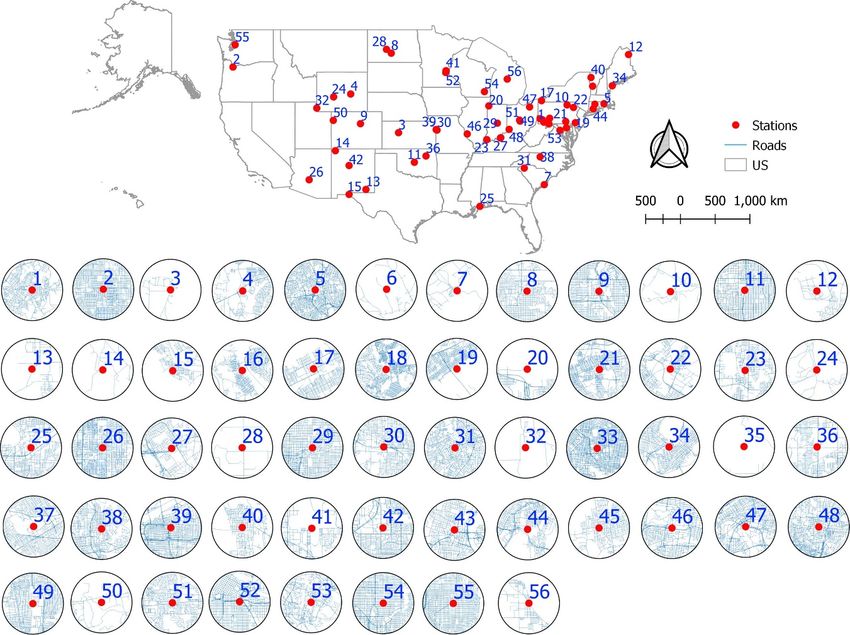
of the element, w implies the width to control the Figure 2 presents 56 NO2 stations in the US, cover-
speed of the dispersion, and x stands for the distance ing a large geographical space, and table 1 summarizes
4Environ. Res. Lett. 16 (2021) 054064 M S Wong et al
Figure 2. Locations of 56 air quality stations across the United States. Each circular area has a 3 km radius centred at the stations,
which are presented as the red dots with IDs. The densities of the road networks are diverse across the whole area.
Table 1. The station IDs are listed in six different climate types. Table 2. Definitions of the abbreviations used in this study.
No. Climate Station ID No. Abbre. Definition
1 Costal 5, 7, 19, 20, 25, 33, 34, 44, 53–55 1 ∆d NO2 difference: the predicted NO2
2 Inland 1–4, 6, 8–18, 21–24, 26–32, 35–52, 56 concentration minus the observed
3 Arid 3, 4, 8, 9, 11, 13–15, 24, 26, 28, 32, NO2 concentration at a station after
42, 50 lockdown
4 Humid 1–2, 5–7, 10, 12, 16–23, 25, 27, 29–31, 2 e relative error: ∆d divided by the
33–41, 43–49, 51–56 observed NO2 concentration
5 Hot 1–3, 5–7, 10, 11, 13–23, 25–27, 29–31, 3 ∆c NO2 change: the mean NO2 concen-
33, 35–39, 42–44, 46–49, 51, 53, 55 tration after lockdown minus that
6 Cold 4, 8, 9, 12, 24, 28, 32, 34, 40, 41, 45, 50, before lockdown
52, 54, 56 4 ∆cp NO2 change in percentage: ∆c divided
by the mean NO2 concentration
before lockdown
5 ∆m the mean change of urban mobility
six climate types that prevail at the stations according subject to a specific day before lock-
to National Weather Service (2020). The stations are down; {∆mw , ∆mr , ∆mt } are the
located in various micro-environments with different changes of mobility for workplace,
road networks, and they are located in urban or rural recreation, and public transit
areas of those cities that implement lockdown when 6 nnd the number of road intersections
the COVID-19 pandemic becomes quite severe. The 7 cnd the number of the road segments con-
necting at all the intersections
training has been done at each station since June 2014.
8 srd the total length of the road networks
Then, the SARIMAX model is used to predict daily 9 nrd the number of the road segments
NO2 at each station from the start of lockdown to the 10 ∆mrd ∆mrd = srd · ∆mw
end of lockdown.
Two predictions are made, with one prediction
period starting 60 days (n = 60) before the lockdown ending a number of days after the lockdown. Figure 3
and ending a number of days after the lockdown visualizes prediction results of two selected sites that
(until 6 May 2020), and the other prediction period the red curves (observation) present a seasonal and
is starting 30 days (n = 30) before the lockdown and periodical pattern, which are lower than the blue
5Environ. Res. Lett. 16 (2021) 054064 M S Wong et al
Figure 3. Prediction of the two selected sites. (a) Site located at Del Norte, New Mexico. (b) Site located at Greenville, South
Carolina.
curves (prediction). The difference between the blue Besides, both errors for n = 30 are slightly smaller
and red curves (i.e. NO2 difference) confirms our than that for n = 60, probably because n = 60 has a
hypothesis that the prediction has not incorporated longer prediction time while n = 30 allows an addi-
the disruption of lockdown and can be explained by tional 30 day training that better incorporates the
the reduction of mobility. most recently seasonal variation into the prediction.
Figure 4(a) provides the distribution of the mean To probe into the impact of the lockdown meas-
relative errors (e) of the prediction at all the stations. ures, in the present study, the NO2 changes before
Evidently, the errors before lockdown (b) are smaller and after lockdown for the 56 stations based on
than after lockdown (a), with the medians at e = 0.13 prediction (p) and observation (o) are calculated,
for n = 60 and e = 0.12 for n = 30, respectively. It sug- respectively. It is found that many stations have
gests that satisfactory prediction accuracy is achieved undergone a substantial reduction after lockdown
prior to the lockdown accordingly. When the lock- in view of the changes of absolute values (∆c)
down was activated, the medians become larger at (figure 4(b)), which become more significant when
e = 0.22 for n = 60 and e = 0.20 for n = 30, which conversion into percentages that ∆cp equals ∆c
indicates that it is challenging to obtain accurate divided by the mean concentration before lockdown
prediction caused by disruptive lockdown measures. (figure 4(c)). Specifically, the observation suggests
6Environ. Res. Lett. 16 (2021) 054064 M S Wong et al
Figure 4. Relative errors of NO2 prediction and statistics of NO2 change. The numbers in each plot are the medians of statistics at
the 50th percentile. The training has been implemented since 2014 at each station and the two predictions start from 60 days
(n = 60) and 30 days (n = 30) before the lockdown dates. (a) Relative errors of the predicted NO2 concentrations (e) at the 56
stations respectively before (b) and after (a) lockdown. (b) NO2 changes (∆c) obtained from prediction (p) and observation (o).
(c) NO2 changes in percentage (∆cp ) obtained from prediction (p) and observation (o).
Figure 5. Changes of urban mobility and NO2 difference in each individual city. (a) Absolute decrease of urban mobility for
workplace (|∆mw |). (b) NO2 change (∆c) after lockdown, corresponding to the city in the x-axis of (a).
that half of the NO2 measurements decreased at least tiny increase is found in four cities quite unexpectedly
with −1.45 mg m−3 for n = 30 and −2.41 mg m−3 (figure 5(b)). Notably, the changing trend of |∆mw |
for n = 60 (figure 4(b)), which is equivalent to a is unclear with the decrease of ∆c, which stimulates
23.08% and 30.38% reduction of the NO2 concen- our motivation to explore the influential factors.
tration before lockdown. Meanwhile, the predicted
number is slightly larger than the observation. 3.2. Association between urban mobility and NO2
According to the COVID-19 Community Mobil- difference
ity Reports from Google that provides relative urban Considering the vehicle emission is one of the largest
mobility subject to a baseline before lockdown in each resources of NO2 , a significant reduction of urban
city, all the involved cities have shown a huge decrease mobility during the pandemic is supposed to have
in the mobility for workplace with |∆mw | > 20%, impacts on the changes of NO2 in cities, which
in which Seattle, Ashburn, Burlington, and Min- focuses on a detailed investigation by contrast with
neapolis have witnessed the largest reduction with other studies at regional and national scales. Based
|∆mw | equalling 41%, 38%, 36%, and 33%, respect- on the COVID-19 Community Mobility Reports, the
ively (figure 5(a)). By inspecting each station, the Pearson correlation analysis between the NO2 differ-
observation suggests that a considerable reduction of ence (∆d) and the averaged mobility changes (∆m)
NO2 after lockdown is realized in most cities, while a is made, in categories of n = 30 (figure 6(a)) and
7Environ. Res. Lett. 16 (2021) 054064 M S Wong et al Figure 6. The Pearson correlation coefficients (R) and the significance (p) between the changes of the three mobilities (∆m) and NO2 difference (∆d) after lockdown. (a) Correlations obtained from n = 30. (b) Correlations obtained from n = 60. Figure 7. Pearson correlation coefficient (R) between ∆d and three indices to represent innate characteristics of road networks. The buffer areas represent the confidence intervals. (a) The number of the road intersections nnd . (b) The total number of road segments connecting at all the intersections cnd . (c) The total length of road networks srd . n = 60 (figure 6(b)). It shows that the mobility for helps reduce urban mobility for recreation, transit, workplace decreases significantly in all cities (−40% ⩽ and workplace greatly during the pandemic, lead- ∆mw ⩽ −15%), which validates a moderate and neg- ing to a considerable reduction of NO2 . Secondly, ative correlation with ∆d in both groups (the Pearson the correlations between ∆m and ∆d, even though correlation coefficient R =−0.47, p
Environ. Res. Lett. 16 (2021) 054064                                                                                           M S Wong et al

   Figure 8. Pearson correlation coefficient (R) between the four indices of road networks (cnd , nnd , srd , nrd ) and ∆d. w in the x-axis
   represents the width of the Gaussian function used to estimate the impact of the four indices on weather stations, and R in the
   y-axis has p ⩽ 0.01. (a)–(d) Correlations are based on n = 30 and n = 60.

i and ∆d, categorizing into two groups of n = 30                         while a short distance to the station is related to a
and n = 60. It is pointed out that both groups obtain                    greater amount of NO2 . On the other hand, w = 2.25
somewhat strong and positive correlations that the                       km is an empirical distance that road networks start
coefficients R = {0.54, 0.54, 0.60} for n = 30, resulting                to have a rather weak impact on ∆d.
a better performance than (∆m, ∆d) in figure 6. It
can be explained that a larger indicator in i makes a                    3.4. Impacts of regional climates on NO2
more significant effect on the changes of NO2 after                      concentration
lockdown, suggesting that road networks’ character-                      The present study considers that regional climates can
istics can greatly affect ∆d. However, the three indic-                  also affect the dispersion of NO2 . It is based on the
ators treat intersections and roads with homogeneous                     evidence that air temperatures were used to describe
impacts on the air quality stations, regardless of the                   urban heat islands and climate largely determines the
spatial distance between the roads and stations.                         magnitude of urban heat islands (Zhao et al 2014,
     To make the indices more representative, we used                    Manoli et al 2019). As both air temperatures and NO2
                           ∑
a Gaussian function y = g(A, x, w) to estimate the                       are air properties essentially, NO2 concentrations may
dispersion of NO2 from the vehicle emission, in which                    also be influenced by climate. To explore the com-
A represents the magnitude of the road property, x                       bined impacts of urban mobility and road networks
denotes the distance from roads to the NO2 station,                      in partition of different climates, the correlation ana-
and w indicates the width of the function. In addi-                      lysis is performed in different climates, namely, arid
tion, another road index named nrd is initiated, which                   and humid climates, hot and cold climates, and coastal
means that the dispersion associated with the road                       and inland climates (figure 9(a)). The correlation
follows the Gaussian distribution but ignoring the                       analysis is performed between ∆d and ∆mrd = srd ·
characteristics of the road length to compare with                       ∆mw , where srd follows the Gaussian function with
the performance of srd . Figure 8 shows the coefficient                  w = 3 km that obtains the largest R and ∆mw is the
curves between i = {nnd , cnd , srd , nrd } and ∆d, com-                 change of workplace mobility as discussed in figure 6.
paring between n = 30 and n = 60. Overall, all the                       Generally, results obtained from n = 30 (figures 9(b)–
curves grow steadily and approach the upper bounds                       (d)) and n = 60 (figures 9(e)–(g)) are almost the same
gradually with an increase of w. Particularly, cnd and                   that (∆d, ∆mrd ) are strongly correlated. Particularly,
nnd share the same growing trend with the increase                       the correlations are more prominent in the arid, hot,
of w that their Rmax < 0.55 (figures 8(a) and (b)).                      and coastal climates with R = {−0.84, −0.65, −0.77}
Also, cnd is insignificantly larger than nnd with the                    than in the humid, cold, and inland climates, namely
same w and the same group n = 30 or n = 60. Com-                         R = {−0.60, −0.64, −0.64} (figures 9(b)–(d)). In
paratively, srd and nrd perform better than cnd and                      contrast, correlations based on n = 60 are slightly
nnd regarding the correlation coefficients R. Mean-                      weaker than n = 30. That is to say, the arid, hot, and
while, srd overtakes nrd notably for both n = 30 and                     coastal climates tend to facilitate the dispersion of
n = 60, and srd shows the most prominent correlation                     NO2 based on a given urban mobility and road net-
with Rmax ≈ 0.60 when w = 3 km (figures 8(c) and                         works. It is also found that ∆mrd shows the most
(d). Two phenomena can be observed from the figure.                      prominent correlation with ∆d, and the significance
On the one hand, srd obtains the strongest impact on                     of the correlations decreases from ∆mrd with the
∆d, which is convincing since srd incorporates the                       Gaussian distribution, srd with the Gaussian distribu-
NO2 source from roads and NO2 dispersion follow-                         tion (figure 8(d)), srd (figure 7(c)), to ∆mw (figure 6)
ing the Gaussian distribution into the correlation. For                  when they are in the same condition. It suggests
instance, a long road is likely to produce more NO2                      that the dynamic mobility constraint by static road

                                                          9
Environ. Res. Lett. 16 (2021) 054064 M S Wong et al
Figure 9. Pearson correlation coefficient (R) between ∆d and ∆mrd estimated by the Gaussian function (w = 3 km). The buffer
areas symbolize the confidence intervals. (a) Stations are located at a place with six types of the climate. (b)–(d) R is derived from
n = 30. (e)–(g) R obtained on the condition of n = 60. (b), (e) Stations are in the arid and humid climates. (c), (f) Stations are in
the hot and cold climates. (d), (g) Stations are in the coastal and inland climates.
networks significantly affects the changes of NO2 in observation. The study also suggests that the pro-
a large geographical space. posed prediction and analysis method can be used to
evaluate the environmental impacts when confront-
4. Discussion and conclusion ing the COVID-19 pandemic and other public health
events.
An accurate estimation of the time series of NO2 The results suggest that part of the difference
is essential to predict and investigate the impact between predicted and observed values is the result of
of the community mobility on the urban micro- the disruptive lockdown measures. During the lock-
environment. The study refines an established NO2 down period, there are strong and negative correla-
prediction model and estimates the NO2 concentra- tions between ∆d and ∆mrd in group of different cli-
tions without the disruption of COVID-19, which mates because ∆mrd considers the changes of urban
is achieved by incorporating the seasonal and cyc- mobility, the total length of the roads, and the dis-
lic variations based on years of historical data before persion following a Gaussian distribution. Two major
2020. Correlation analysis in this study is performed findings have been generalized as follows. Firstly, a
based on the hypothesis that the predicted level of great reduction of urban mobility associated with the
NO2 after lockdown is larger than the observed level recreation, transit, and workplace may result in a con-
because the lockdown policy leads to less frequent siderable decrease in NO2 in a large geographical area.
use of vehicles and thus less NO2 emission while the Secondly, the local climate is also one of the vital
prediction still follows historical patterns that have factors that have distinct impacts on the dispersion
not incorporated the dramatic decrease of NO2 after of NO2 . Specifically, the impacts are more prominent
lockdown. Therefore, the changes of urban mobil- for stations in areas where the arid, hot, and coastal
ity have shown a causal relation with the difference climates prevail, since the three climates’ correlations
of NO2 concentrations between the prediction and are considerably stronger. It is probably because the
10Environ. Res. Lett. 16 (2021) 054064 M S Wong et al
arid and hot climates would cause uneven air temper- Kwon Ho Lee https://orcid.org/0000-0002-0844-
atures, which promotes wind ventilation and reduces 5245
the NO2 density, and it is also the case with coastal cit-
ies where there are wind cycles between the land and
sea. Some features of local weather in terms of daily References
wind directions and strengths can also mitigate NO2
concentrations. Air Quality Open Data Platform 2020 Air pollution in world:
The SARIMAX model considers meteorological real-time air quality index visual map (available at: https://
aqicn.org/map/world/)
conditions by establishing exogenous weather vari-
Brauer M 2010 How much, how long, what and where: air
ables, such as wind speed and air pressure, optim- pollution exposure assessment for epidemiologic studies of
ized by minimizing the AIC value to achieve accur- respiratory disease Proc. American Thoracic Society vol 7
ate prediction. Since this study aims to investigate pp 111–15
Carslaw D C 2005 Evidence of an increasing NO2/NOx emissions
the impacts of mobility on NO2 concentration, we
ratio from road traffic emissions Atmos. Environ.
do not analyse the meteorological influence in detail. 39 4793–802
Alternatively, we have categorized the analysis into six Chan T L et al 2004 On-road remote sensing of petrol vehicle
climate types, which is used as background climate emissions measurement and emission factors estimation in
Hong Kong Atmos. Environ. 38 2055–66
associating with meteorological conditions, to obtain
Cohen A J et al 2017 Estimates and 25-year trends of the global
generic phenomenon at a large geographical extent. burden of disease attributable to ambient air pollution: an
The prediction with 30 and 60 days before lockdown analysis of data from the global burden of diseases study
suggests that instantly seasonal variation influences 2015 Lancet 389 1907–18
Congressional Research Service 2020 Global economic effects of
prediction accuracy, while their effect is insignificant
COVID-19 (available at: https://fas.org/sgp/crs/row/
when associating with mobility indicators to explain R46270.pdf)
NO2 concentration. Earth Observatory 2020 Airborne nitrogen dioxide plummets
In conclusion, the proposed NO2 difference (available at: https://earthobservatory.nasa.gov/images/
146362/airborne-nitrogen-dioxide-plummets-over-china)
between prediction and observation is an effective
Fan J L et al 2020 How do weather and climate change impact the
indicator to explain the improvement of the air qual- COVID-19 pandemic? Evidence from the Chinese mainland
ity after lockdown. The proposed ∆mrd can explain Environ. Res. Lett. 16 014026
the NO2 concentration comprehensively by consider- Faranda D et al 2015 Early warnings indicators of financial crises
via auto regressive moving average models Commun.
ing the source of dynamic urban mobility, the spatial
Nonlinear Sci. Numer. Simul. 29 233–9
constraints of road networks, and physical dispersion Google 2020 COVID-19 community mobility reports (available
process. The proposed analysis method can be used to at: https://google.com/covid19/mobility/)
investigate other air quality indicators and other dis- Greenberg N et al 2016 Different effects of long-term exposures to
SO2 and NO2 air pollutants on asthma severity in young
ruptive infectious diseases.
adults J. Toxicol. Environ. Health A 79 342–51
Guan D et al 2020 Global supply-chain effects of COVID-19
Data availability statement control measures Nat. Hum. Mobility 4 557–87
Haiges R, Wang Y D, Ghoshray A and Roskilly A P 2017
The data that support the findings of this study are Forecasting electricity generation capacity in Malaysia: an
auto regressive integrated moving average approach Energy
available upon reasonable request from the authors.
Proc. 105 3471–8
He Q et al 2020 Spatially and temporally coherent reconstruction
Acknowledgments of tropospheric NO2 over China combining OMI and
GOME-2B measurements Environ. Res. Lett. 15 125011
Heeb N V, Saxer C J, Forss A M Brühlmann S 2008 Trends of NO-,
Man Sing Wong thanks the funding support from NO2 - and NH3-emissions from gasoline-fueled Euro-3-to
a grant by the General Research Fund (Grant No. Euro-4-passenger cars Atmos. Environ. 42 2543–54
15602619), and the Research Institute for Sustain- Hueglin C, Buchmann B and Weber R O 2006 Long-term
observation of real-world road traffic emission factors
able Urban Development (Grant No. 1-BBWD), the on a motorway in Switzerland Atmos. Environ. 40
Hong Kong Polytechnic University. Mei-Po Kwan 3696–709
was supported by a grant from the Research Com- Hyndman R J and Khandakar Y 2008 Automatic time series
mittee on Research Sustainability of Major RGC forecasting: the forecast package for R J. Stat. Softw.
27 107590
Funding Scheme of the Chinese University of Hong Kendrick C M, Koonce P and George L A 2015 Diurnal and
Kong. This research is supported by the National seasonal variations of NO, NO2 and PM2.5 mass as a
Research Foundation, Prime Minister’s Office, Singa- function of traffic volumes alongside an urban arterial
pore under its Campus for Research Excellence and Atmos. Environ. 122 133–41
Keuken M, Roemer M and van den Elshout S 2009 Trend analysis
Technological Enterprise (CREATE) programme. of urban NO2 concentrations and the importance of direct
NO2 emissions versus ozone/NOx equilibrium Atmos.
ORCID iDs Environ. 43 4780–3
Khaniabadi Y O et al 2017 Exposure to PM10 , NO2 and O3 and
impacts on human health Environ. Sci. Pollut. Res.
Rui Zhu https://orcid.org/0000-0002-9965-0948
24 2781–9
Coco Yin Tung Kwok https://orcid.org/0000- Kucharski A J, Russell T W, Diamond C, Liu Y and Edmunds J
0001-6886-3281 2020 Early dynamics of transmission and control of
11Environ. Res. Lett. 16 (2021) 054064 M S Wong et al
COVID-19: a mathematical modelling study Lancet Shon Z H, Kim K H and Song S K 2011 Long-term trend in NO2
Infectious Dis. 20 553–8 and NOx levels and their emission ratio in relation to road
Kurtenbach R, Kleffmann J, Niedojadlo A and Wiesen P 2012 traffic activities in East Asia Atmos. Environ. 45 3120–31
Primary NO2 emissions and their impact on air quality in Shrestha A M et al 2020 Lockdown caused by COVID-19
traffic environments in Germany Environ. Sci. Eur. 24 21 pandemic reduces air pollution in cities worldwide
Lakhani A 2020 Which Melbourne metropolitan areas are EarthArXiv (https://doi.org/10.31223/osf.io/edt4j)
vulnerable to COVID-19 based on age, disability and access Singer G, Zivin J G, Neidell M and Sanders N 2020 Air pollution
to health services? Using spatial analysis to identify service increases influenza hospitalizations medRxiv (https://
gaps and inform delivery J. Pain Symptom Manage. 60 41–4 doi.org/10.1101/2020.04.07.20057216)
Lee C 2019 Impacts of urban form on air quality in metropolitan Singh S N and Mohapatra A 2019 Repeated wavelet transform
areas in the United States Comput. Environ. Urban Syst. based ARIMA model for very short-term wind speed
77 101362 forecasting Renew. Energy 136 758–68
Liu L J S et al 2012 Long-term exposure models for traffic related State Space Methods 2020 Seasonal AutoRegressive integrated
NO2 across geographically diverse areas over separate years moving average with eXogenous regressors model (available
Atmos. Environ. 46 460–71 at: https://statsmodels.org/dev/generated/
Mahato S, Pal S and Ghosh K G 2020 Effect of lockdown amid statsmodels.tsa.statespace.sarimax.SARIMAX.html)
COVID-19 pandemic on air quality of the megacity Delhi, Tang J et al 2019 Assessing the impact of vehicle speed limits and
India Sci. Total Environ. 730 139086 fleet composition on air quality near a school Int. J. Environ.
Manoli G et al 2019 Magnitude of urban heat islands largely Res. Public Health 16 149
explained by climate and population Nature 573 55–60 UN News 2020 UN launches COVID-19 plan that could ‘defeat
Meng X et al 2015 A land use regression model for estimating the the virus and build a better world’ (available at: https://
NO2 concentration in Shanghai, China Environ. Res. news.un.org/en/story/2020/03/1060702)
137 308–15 Valipour M 2015 Long-term runoff study using SARIMA and
Minoura H and Ito A 2010 Observation of the primary NO2 and ARIMA models in the United States Meteorol. Appl.
NO oxidation near the trunk road in Tokyo Atmos. Environ. 22 592–8
44 23–9 Velders G J and Diederen H S 2009 Likelihood of meeting the EU
Mohegh A, Goldberg D, Achakulwisut P and Anenberg S C 2020 limit values for NO2 and PM10 concentrations in the
Sensitivity of estimated NO2 -attributable pediatric asthma Netherlands Atmos. Environ. 43 3060–9
incidence to grid resolution and urbanicity Environ. Res. Venter Z S, Aunan K, Chowdhury S Lelieveld J 2020 COVID-19
Lett. 16 014019 lockdowns cause global air pollution declines PNAS
National Weather Service 2020 Addition Köppen-Geiger climate 117 18984–90
subdivisions (available at: https://weather.gov/jetstream/ Wang Y et al 2020 Spatial decomposition analysis of NO2 and
climate_max) PM2.5 air pollution in the United States Atmos. Environ.
Open Weather 2020 We deliver 2 billion forecasts per day 241 117470
(available at: https://openweathermap.org/) Zhao L, Lee X, Smith R B and Oleson K 2014 Strong
OpenStreetMap 2020 A map of the world under an open license contributions of local background climate to urban heat
(available at: https://openstreetmap.org) islands Nature 511 216–19
Palmgren F, Berkowicz R, Ketzel M and Winther M 2007 Elevated Zhu Y, Jingu X, Fengming H and Liqing C 2020 Association
NO2 pollution in Copenhagen due to direct emission of between short-term exposure to air pollution and
NO2 from road traffic 2nd ACCENT Symp. (Urbino, Italy, COVID-19 infection: evidence from China Sci. Total
23–27 July) Environ. 727 138704
12You can also read