AstroMHD@HZDR Frank Stefani
←
→
Page content transcription
If your browser does not render page correctly, please read the page content below
AstroMHD@HZDR
Frank Stefani
Text optional: Institutsname Prof. Dr. Hans Mustermann www.fzd.de Mitglied der Leibniz-Gemeinschaft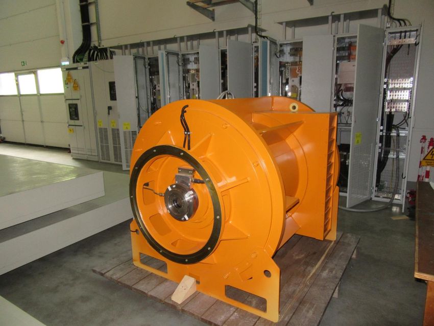
Two (interrelated) reasons to initiate „AstroMHD“…
New projects with new PhD students (…and 2 Postdocs)

1. ERC project LEMAP (Federico, Jude, N.N., N.N., George,… )
2. Helmholtz-Russian Science Foundation project „Magnetohydrodynamic
   instabilities…“ (Peter, Sebastian)
3. André´s DFG project on precession with blades (N.N.)
4. Rayleigh-Bénard activities…
POF 4 (2021-2027): Transfer of activities from research field „Energy“ into
research field „Matter“, Program „From matter to materials and live (MML)“

1. DRESDYN precession dynamo
2. DRESDYN MRI/TI experiment
3. Rayleigh-Bénard activities ???

…first draft until 19 March 2019!!!,
 strategic evaluation: 27-39 January 2020
Seite 2
AstroMHD is intended…

• …to be an open forum for project discussions with focus on the projects
  with geo- and astrophysical relevance
• …for detailed discussion of data from the related experiments and/or
  numerical models, or technical challenges that are crucial for the
  configurations of experimental and numerical setups
• …in rare cases (as today) for lectures

 AstroMHD is not intended…

• …to replace the Coffee Meetings
• …as a series of lectures on basic MHD

Seite 3
Astrophysical MHD: Motivation
                         Cosmic magnetic fields…
     …are produced by the                     …play a key role in cosmic structure
     homogeneous dynamo effect                formation by virtue of the
                                              magnetorotational instability

          Rüdiger, Kitchatinov, Hollerbach:
          Magnetic Processes in Astrophysics (2013)

Seite 4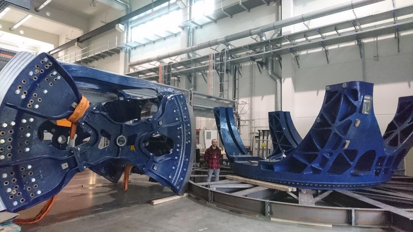
Astrophysical MHD: Basic mechanisms

 Homogeneous dynamo effect:           Magnetorotational instability (MRI):
 Self-excitation of magnetic fields   Magnetic fields act like springs and
 in sufficiently strong, helical      trigger angular momentum transport in
 flows of conducting fluids           accretion disks around protostars or
                                      black holes

Seite 5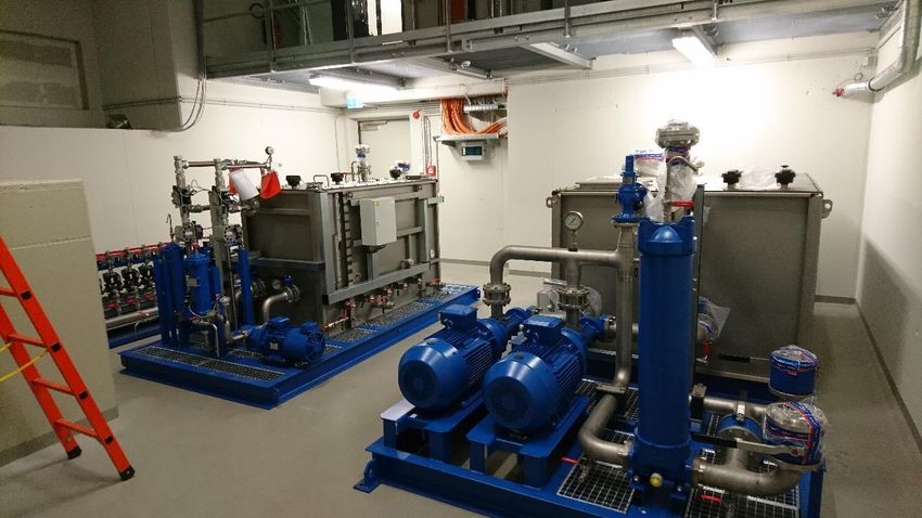
Astrophysical MHD: Underlying theory
u P curl B B
Navier-Stokes equation: u u 2u
t 0
Governing parameters: LV
Re Ha BL
(Reynolds, Hartmann)
B 1
Induction equation: curl (u B) 2B
t 0
Governing parameter:
Rm 0LV
(magnetic Reynolds)
Seite 6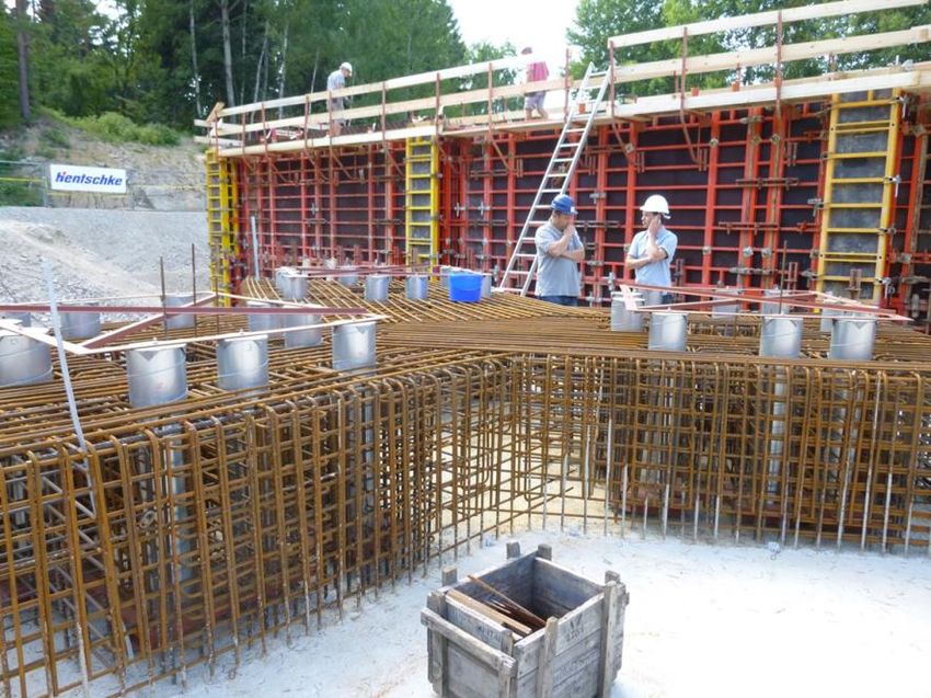
Astrophysical MHD: Previous, present, and future experiments

Seite 7
DREsden sodium facility for DYNamo and thermohydraulic studies
     • DRESDYN building ~500 m2
     • Total sodium inventory: 12 tons
     • Precession driven dynamo experiment with separate
       strong basement and containment for Argon flooding
     • Large experimental hall for MRI/TI experiment, sodium
       loop, liquid metal batteries, Rayleigh-Bénard experiment

      Stefani et al.: Magnetohydrodynamics 48 (2012), 103; 51
      (2015), 275; Geophys. Astrophys. Fluid Dyn. (2018)
Seite 8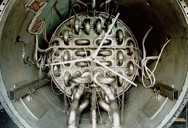
The Yin-Yang of astrophysical MHD

          First                      Third
          part                       part

                                      Second
                                      part
Design by M. Seilmayer
Seite 9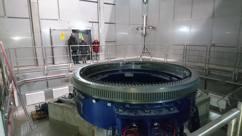
Dynamos

       First
       part

Seite 10
Matter under extreme conditions Requires large sodium facilities
Why sodium? Condition for magnetic self-excitation: Magnetic Reynolds
number must be larger than ~10:
Rm = μσUL > Rmcrit 10
( - magnetic permeability, - conductivity, U - tyical velocity, L- typical size)
Sodium is the best liquid conductor with σ~107 S/m UL~1 m2/s
Why so large? Necessary power scales with 1/L:
P ~ Rm3 / L
Reasonable motor power (a few 100 kW) only with large facilities (~1 m)
Seite 11Some history: Riga dynamo experiment Seite 12
Riga dynamo experiment
 First experimental realization of magnetic
 field self-excitation in a liquid metal flow
 (11 November 1999)

 Gailitis et al., Phys. Rev. Lett. 84 (2000) 4365; Phys. Rev. Lett. 86
 (2001) 3024; Rev. Mod. Phys. 74 (2002) 973 ; Phys. Plasmas 11
 (2004) 2838; Compt. Rend. Phys. 9 (2008), 721
Seite 13
Riga dynamo – Attention: Sodium!

           Evening of 11th
           November 1999...

                                    …and the day after...

Seite 14
Riga dynamo experiment From the kinematic to the saturated regime (July 2000) Gailitis et al., Phys. Rev. Lett. 84 (2000) 4365; Phys. Rev. Lett. 86 (2001) 3024; Rev. Mod. Phys. 74 (2002) 973 ; Phys. Plasmas 11 (2004) 2838; Compt. Rend. Phys. 9 (2008), 721 Seite 15
Riga dynamo experiment
 Switching the dynamo on and off
 (February 2005)

 Gailitis et al., Phys. Rev. Lett. 84 (2000) 4365; Phys. Rev. Lett. 86
 (2001) 3024; Rev. Mod. Phys. 74 (2002) 973 ; Phys. Plasmas 11
 (2004) 2838; Compt. Rend. Phys. 9 (2008), 721
Seite 16
Riga dynamo experiment: Growth rates and frequencies

             Numerical predictions (with correct vacuum boundary conditions)
             of the kinematic dynamo were accurate to some 5-10 per cent
             Simplified back-reaction model (Lorentz forces acting along
             streamlines) gives very reasonable field amplitudes and structures
             in the saturation regime
           Gailitis et al., C. R. Physique 9 (2008), 721;
           J. Plasma Phys. 84, 735840301 (2018)
Seite 17
Some history: Karlsruhe Dynamo Experiment
A two-scale, a2 type dynamo,
realized by 52 spin-generators
Stieglitz and Müller, Phys. Fluids 13, 561 (2001)
Seite 18Karlsruhe Dynamo Experiment
Again, very good agreement
with numerical predictions
Rädler et al. Nonl. Proc. Geophys. 9,
(2002), 171
„Secret Fax“ of 19 December 1999
Seite 19„Dynamo Riga“ versus „Dynamo Karlsruhe“ Seite 20
Some history: von-Karman-Sodium (VKS) Experiment in Cadarache

VKS has shown self-excitation and a wealth of wonderful dynamical effects,
including oscillations, reversals, burst, localized fields….

                                Monchaux et al., Phys. Fluids 21 (2009), 035108

Seite 21
VKS-Dynamo: Role of high impellers?
…on the basis of the dominant toroidal mode,
some small-scale helicity between the blades
(a-effect) is sufficient to ignite the dynamo
Giesecke et al., Phys. Rev. Lett. 104 (2010); New J.
Phys. 14 (2012), 053005
Nore et al., Europhys. Lett. 114 (2016), 65002
Kreuzahler et al, Phys. Rev. Lett. 119 (2017), 234501
Seite 22Reversals of the geomagnetic field and the VKS dynamo field
Berhanu et al., EPL 77 (2007), 59001
Seite 23The DRESDYN precession dynamo: Geo/astrophysical motivation
Strong indication for influence of variations of
Earth‘s orbit parameters on the geodynamo
Probability density of inter-
reversal times shows
maxima at multiples of the
Milankovic cycle of Earth‘s
orbit eccentricity (95 ka)
climate??
Doake, Nature 267 (1977), 415
Consolini, De Michelis, Phys. Rev. Lett. 90 (2003), 058503
Recent discussion of the lunar dynamo in terms of precession or impacts
Dwyer et al., Nature 479 (2011), 212; Le Bars et al., Nature 479 (2011), 215
Evidence for ancient core dynamo in asteroid Vesta
Fu et al., Science 338 (2012), 238
Seite 24Precession driven dynamo experiment within the DRESDYN project Key parameters: • Cylinder with 2 m diameter and 2 m height, 8 tons of liquid sodium • Cylinder rotation: 10 Hz (will need some 800 kW motor power) • Turntable rotation: 1 Hz • Magnetic Reynolds number ~ 700 • Gyroscopic torque onto the basement: 8 MNm ! Seite 25
“Fundamental” problems due to huge gyroscopic torque
April 2013: drilling 7 holes (22 m deep)
July 2013: Constructing the
ferroconcrete basement
May 2015: The tripod for the
dynamo within the containment
(with stainless steel “wallpaper”)
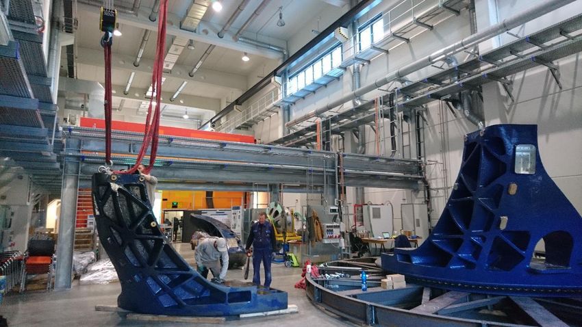
Seite 26Precession driven dynamo: Underframe mounted on tripod (3/2018) Seite 27
Precession driven dynamo: Large ball bearing installed (12/2018)

Seite 28
Precession driven dynamo: Traverse and pylons (01/2019)

Seite 29
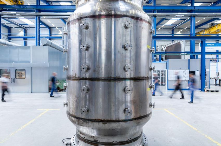
Precession driven dynamo: Central vessel welded

Seite 30
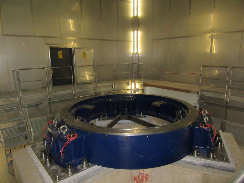
Precession driven dynamo: Motor for rotation is tested

Seite 31
Precession driven dynamo: Oil station for ball bearings (12/2018)

Seite 32
Precession driven dynamo: Motor for turntable rotation (01/2019)

Seite 33
Precession driven dynamo: Sodium tanks; piping system is designed

Seite 34
Test of the fire extinguishing facility with liquid argon (01/2016)

Seite 35
Precession driven dynamo experiment: our plan for 2019...

Seite 36
Precession driven flow: Will it really be a dynamo?

  New encouraging result:

  Axisymmetric double-roll flow
  (s2t1) emerges in the nonlinear
  regime from the forced m=1 Kelvin
  mode in a (narrow) region of the
  precession ratio.

  Possible explanation: The
  modified rotational profile
  becomes Rayleigh-unstable and
  develops 2 Taylor vortices.

  Shortly beyond that, the flow
  becomes turbulent

                                          Giesecke et al., Phys. Rev. Lett. 120
                                          (2018), 024502
Seite 37
Precession driven dynamo: Realistic prospects for self-excitation
• Remarkable agreement of numerics and experiment for Re=10000
• Experiment shows: double-roll flow remains robust for higher Re
• In a narrow range of the precession ratio, dynamo is predicted for
Rm~430 (Rm=700 is technically feasible)
Giesecke et al., Phys. Rev. Lett. 120
(2018), 024502
Seite 38Schedule for precession experiment • 14 March: pressure test of the rotation vessel (with 35 bars) • 5 June: delivery of rotation vessel to HZDR • 26 August: large slip-ring installed • 7 November: rotation vessel mounted on the platform After that: • test of all systems • dry rotation (also for calibrating strain gauges) • 2020: water experiments • 2021…: sodium experiments Seite 39
Next steps for us… 1. Preparing the first water-experiments (to start in early 2020): André, Thomas, Tobias, Matthias, N.N. next meeting 19 March 2. Simulations for different nutation angles: Federico, Jan Simkanin 3. Experiments and simulations for the case with inserted blades (André´s DFG project) 4. Securing the dynamo predictions by simulations with vacuum boundary conditions 5. Enhancing SEMTEX by induction equations in order to simulate a dynamically consistent dynamo Seite 40
Magnetorotational and Tayler instability

                                            Second
                                            part

Seite 41
How do accretion discs work?
Central object (protostar, black hole)
Accretion disk
• Problem: Outward angular momentum transport is not
explainable by normal viscosity
• Turbulence could help. But: Kepler rotation is hydrodynamically
stable. Where does the turbulence come from?
Seite 42History of MRI: Magnetized Tayler-Couette flow E.P. Velikhov: Sov. Phys. JETP 9 (1959), 995 Rüdiger, Gellert, Hollerbach, Stefani, Phys. Rep. 741, 1 (2018) Seite 43
(Citation) history of MRI

                            182                        2689

           The discoverer (1959)        The adopters (1991)
           E.P. Velikhov: Sov. Phys.   S.A. Balbus and J.F. Hawley:
           JETP 9 (1959), 995          ApJ 376 (1991), 214

Seite 44
Standard MRI and helical MRI
• Standard MRI (with purely axial field) scales
with Lundquist (S) und magnetic Reynolds
(Rm)
• Experiments on SMRI with large Rm in
Maryland and Princeton DRESDYN
• Helical MRI: Bz replaced by Bz+Bj: scales
with Hartmann (Ha) and Reynolds (Re)
Hollerbach and Rüdiger: Phys. Rev.
Lett. 95 (2005), 124501
• Recrit: 103 instead of 106
• Hacrit: 30 instead of 1000
• Potsdam ROssendorf Magnetic InStability
Experiment (PROMISE)
• Drawback: does not work for Kepler (yet)!
Seite 45Helical magnetorotational instability (HMRI) 2006: First experimental evidence of HMRI Stefani et al., Phys. Rev. Lett. 97 (2006), 184502; New J. Phys. 9 (2007), 295; Phys. Rev. E 80 (2009), 066303 Seite 46
HMRI: Experimental evidence, and good agreement with theory

   Example: Increase of central current (i.e, of Bj, and b)

                    Stefani et al., Phys. Rev. E 80 (2009), 066303

Seite 47
Azimuthal MRI (AMRI): m=1 mode under influence of dominant Bj
Hollerbach, Teeluck, Rüdiger:
Phys. Rev. Lett. 104 (2010), 044502 Power supply for 20 kA
Very important: Numerical simulation of the real geometry, including the slight
symmetry breaking of the applied magnetic field
Seite 48Evidence for AMRI: m=1 mode under influence of (nearly) pure Bj Very important: Simulation of real geometry (V. Galindo) Seilmayer et al., Phys. Rev. Lett. 113 (2014), 024505 Seite 49
New results show effect of convection on mode selection of AMRI

                                                    Heating from inside

                 Heating from outside

   Seilmayer et al., PAMIR conference proceedings
Seite 50
Instabilities in spherical Couette experiment (HEDGEHOG)
New results on modulated waves
in HEDGEHOG
2 April, Talk by Ferran
Seite 51Kink-type Tayler instability (TI)
Astrophysical motivation:
• Alternative mechanism of solar
dynamo (Tayler-Spruit dynamo)
• Braking of neutron stars
• Structure formation in cosmic jets
Seilmayer et al.,
Phys. Rev. Lett. 108
(2012), 244501
Seite 52Tayler-Spruit dynamo: Experimental and numerical results for TI
Experiment Numerics
Weber et al., New J.
Phys. 15 (2013), 043034
Seilmayer et al., Phys. Rev. Lett. 108 (2012), 244501
Seite 53Relevance of TI (and other instabilities) for liquid metal batteries? Stefani et al., Energy Conv. Managem. 52 (2011), 2982; Weber et al., J. Power Sources 265 (2014), 166; Stefani et al. IOP Conf. Ser.: Mater. Sci. Eng. 143 (2016), 012024 Seite 54
Combined MRI/TI experiment planned in the framework of DRESDYN

 ...will (hopefully) allow us to study helical MRI, azimuthal MRI, standard MRI,
 and their combinations with Tayler instability

     • Rin=0.2 m
     • Rout=0.4 m
     • H=2 m

     • fin=20 Hz
     • fout=6 Hz

     • Bz=120 mT
     • (will need
       some 110 kW)

     • Rm=40
     • Lundquist=8

Seite 55
Combined MRI/TI experiment: (nearly) final design Seite 56
Combined MRI/TI experiment: test of magnetic coupler

Seite 57
First test failed with a crash at 1000 rpm! Repair is finished...

Seite 58
Basic problem: Are rotational flows with positive shear always stable?
Deguchi, Phys. Rev. E
95 (2017), 021102        HERE: Prospects for
                         magnetic destabilization   Possible
Non-axisymmetric                                    relevance for the
purely hydrodynamic                                 equator-near
instability for Re~107                              parts of the solar
                                                    tachocline

           ???

Seite 59
Can magnetic fields destabilize rotational flows with positive shear?
r
Ro
2 r
r A
Rb
2 A r
Kirillov and Stefani,
Phys. Rev. Lett. 111
(2013), 061103; JFM
Lower Liu Limit Upper Liu Limit 760 (2014), 591
Liu, Goodman, Herron, Ji, Phys. Rev. E 74 (2006), 056302
Seite 60Link between non-modal growth and dissipation-induced instabilities
Any physical reason for the
lower and upper Liu limits (LLL
and ULL) of the shear for the
emergence of HMRI?
YES!
Analytical link between non-
modal growth factor G of
purely hydro-dynamic flows
with modal growth rate g of
dissipation-induced HMRI
Mamatsashvili and Stefani, PRE 94, 051203 (R) (2016)
Seite 61AMRI at positive shear - „Super-AMRI“ - operates at Ro>RoOLL =4.828
Stability curve as a solution of :
Stefani and Kirillov and Stefani, Phys. Rev. E 92 (2015), 051001
Seite 62Super-AMRI also found in 1D-stability analysis
(dashed lines are the
stability boundaries of
Super-AMRI at different
Ωout/Ωin 4,8,128> 1)
Rüdiger et al., Phys. Fluids
(Rüdiger
28 (2016), et al. 16)
014105
Translation of the unstable range Ro>RoULL in the local analysis into the
ratio of outer and inner cylinders‘ angular frequencies for super rotation
Ωout/Ωin > 1 in the global case is crucial!
Taylor-Couette-Experiment with small gap is needed (at least
rin/rout~0.8), Minimum central current ~ 30 kA
Seite 63„Super-AMRI“ experiment with sodium seems feasible
Increasing ratio of wall to fluid conductivity
Ri/Ro=0.9
• Using copper walls, best value for Ri/Ro=0.78: I=33 kA
• This should be doable in a dedicated sodium experiment
Rüdiger et al., Geophys. Astrophys. Fluid Dyn. 112, 301 (2018)
Seite 64Yet, this type of Super-AMRI is a bit frustrating since...
...the upper Liu limit value Ro>RoOLL =4.828 is quite a large positive shear
compared to those found in astrophysical objects or in usual lab
experiments. (for example, the positive shear in the equatorial parts of the
solar tachocline is only Ro~0.5)
Open questions:
Can any sort of HMRI and/or AMRI still survive at astrophysically relevant,
smaller positive shear?
Can such an instability still operate at wider gap width in TC flows
(e.g., for rin/rout~0.5) corresponding to PROMISE and the DRESDYN
MRI/TI experiment
Seite 65What about Super-HMRI? A big suprise…
New mode of HMRI Usual Super- HMRI
Ha 90,
Re 8000,
a 1, b 1
Pm 106
1. A new mode of HMRI: at small k z , all Ro and non-zero (finite) Pm 0
2. Usual Super-HMRI: at larger k , high shear Ro > RoULL , down to the
inductionless limit Pm 0 (dashed black line)
z
Mamatsashvili et al., arXiv:1810.13433
Seite 66The instability domain in the Ro-Pm plane
RoULL 4.828
The stability boundaries at Pmc 2 ( Ro) > 1 (red) and Pmc1 ( Ro) 1 (blue)
are related by
1
Pmc1
Pmc 2
The new double-diffusive HMRI is not constrained by the upper Liu limit.
There is no instability at Pm=1 .
Seite 67Results: 1D Confirmation of WKB result for Pm1 1. Ha and Re (or S and Rm ), as well as k z , increase with b in qualitative agreement with the scalings in the WKB analysis 2. At small Pm 1 , relevant parameters are again the Lundquist, S , and magnetic Reynolds Rm numbers, as in the WKB case Seite 68
Results: Growth rate (optimized over kz) in the (S-Rm) plane
Pm 106
b 1
The unstable region is localized, as in the local analysis, reaching a maximum
value g m 4.8 10 at Sm 5.2, Rmm 25
3
The instability emerges at the minimum Rmc 0.9 and Sc 0.3
Seite 69Prospects for an experiment
Those values S~5 and Rm~25 are well within the capabilities of the
new Taylor-Couette device being currently built within DRESDYN…
• rin=0.2 m
• rout=0.4 m
• h=2 m
• fin=20 Hz
• fout=6 Hz
• Bz=120 mT
• Rm = 40
• S=8
...offering a realistic prospect for experimental realization of this new
double-diffusive, positive shear HMRI
Seite 70Next steps for us… 1. Finalizing the experiments on transition between AMRI and HMRI at PROMISE (with effect of convection): Martin, Jude… meeting on 26 March 2. Finalizing the design of the large MRI/TI experiment: Martin with Sebastian Köppen (FWF) 3. Validating the feasibility of Super-HMRI in the MRI/TI set-up: George+N.N. 4. Optimizing the design of a dedicated Super-AMRI experiment (33 kA minimum!!!) 5. Evaluating the consequences of Super-HMRI for a nonlinear dynamo in the solar tachocline… Seite 71
Nonlinear Tayler-Spruit dynamos (and their tidal synchronization???)

                                                        Third
                                                        part

Seite 72
Solar dynamo models: Basics
Any solar dynamo needs:
• some effect to regenerate toroidal field from poloidal field
• some a effect to regenerate poloidal field from toroidal field
effect a effect
Parker, Astrophys J. 122, 293 (1955)
Seite 73Tayler-Spruit dynamo in the solar tachocline: The main problem
Spruit, Astron. Astrophys. 381 (2002) 923;
Zahn et al., Astron. Astrophys. 474 (2007) 147
Seite 74Tayler instability: Saturation and helicity oscillations at Pm=10-6
(Damped) helicity oscillations Ha =70
u alpha
Ha =100
Weber et al., New J. Phys. 17 (2015), 113013
Seite 75Character of the helicity oscillations
Ha =100
Pm=10-6
Weber et al., New J. Phys. 17 (2015), 113013
Seite 76Planetary tides and the solar cycle: Venus-Earth-Jupiter alignments
Amazing synchronization of solar cycle with the 11.07 years alignment
cycle of the Venus-Earth-Jupiter system (despite tiny tidal forces!)
Bollinger, Proc. Okla. Acad. Sci. 33 (1952), 307; Takahashi, Solar. Phys. 3 (1968), 598;
Wood, Nature 240 (1972), 91; Wilson, Pattern Recogn. Phys. 1 (2013), 147; Okhlopkov,
Mosc. U. Bull. Phys. B. 69 (2014), 257; Okhlopkov, Mosc. U. Bull. Phys. B. 71 (2016),
444; Scafetta, Pattern Recogn. Phys. 2 (2014), 1
Seite 77Planetary tides and the solar cycle: Venus-Earth-Jupiter alignments
Amazing synchronization of solar cycle with the 11.07 years alignment
cycle of the Venus-Earth-Jupiter system (despite tiny tidal forces!)
Sunspots
VEJ index
Bollinger, Proc. Okla. Acad. Sci. 33 (1952), 307; Takahashi, Solar. Phys. 3 (1968), 598;
Wood, Nature 240 (1972), 91; Wilson, Pattern Recogn. Phys. 1 (2013), 147; Okhlopkov,
Mosc. U. Bull. Phys. B. 69 (2014), 257; Okhlopkov, Mosc. U. Bull. Phys. B. 71 (2016),
444; Scafetta, Pattern Recogn. Phys. 2 (2014), 1
Seite 78Planetary tides and the solar cycle: Venus-Earth-Jupiter alignments
Amazing synchronization of solar cycle with the 11.07 years alignment
cycle of the Venus-Earth-Jupiter system (despite tiny tidal forces!)
Sunspots
VEJ index Accident, or
something more…?
Bollinger, Proc. Okla. Acad. Sci. 33 (1952), 307; Takahashi, Solar. Phys. 3 (1968), 598;
Wood, Nature 240 (1972), 91; Wilson, Pattern Recogn. Phys. 1 (2013), 147; Okhlopkov,
Mosc. U. Bull. Phys. B. 69 (2014), 257; Okhlopkov, Mosc. U. Bull. Phys. B. 71 (2016),
444; Scafetta, Pattern Recogn. Phys. 2 (2014), 1
Seite 79Planetary tides and the solar dynamo: The basic 22 years cycle
Amazing synchronization of solar cycle with the 11.07 years conjunction
cycle of the Venus-Earth-Jupiter system (despite tiny tidal forces!)
Schove, D.J.: J. Geophys. Res. 60 (1955), 127; Hathaway, D.H., Liv. Rev. Sol. Phys. 7
(2010), 1; Okhlopkov, Mosc. U. Bull. Phys. B. 71 (2016), 444
Stefani et al., arXiv:1803.08692
Seite 80Dicke´s argument
Distinction between random walk
(RW) and clocked process (CP) for
the instants yn of sunspot maxima
(Dicke) or minima (here):
Residuals: dyn =yn-y0-p(n-1),
with p being the mean cycle period
A telling measure for discriminating
Dicke, R.H., Nature 276 (1978), 676
between RW und CP is the RATIO
between the mean square of dyn and
the mean square of (dyn – dyn-1 )
RATIO Dicke (N=25) Here (N=90)
Random walk (N+1)(N2-1)/3(5N2+6N-3) 1.72 6.12
Clocked process (N2-1)/2(N2+2N+3) 0.46 0.49
Observation 0.87 1.19
Seite 81Dicke´s argument
Distinction between random walk
(RW) and clocked process (CP) for
the instants yn of sunspot maxima
(Dicke) or minima (here):
!!! Residuals: dyn =yn-y0-p(n-1),
with p being the mean cycle period
A telling measure for discriminating
between RW und CP is the RATIO
• After subtraction of Suess/de between the mean square of dyn and
Vries cycle, Dicke‘s ratio fits the mean square of (dyn – dyn-1 )
nearly perfectly to a clocked
process (CP)
RATIO Dicke (N=25) Here (N=90)
Random walk (N+1)(N2-1)/3(5N2+6N-3) 1.72 6.12
Clocked process (N2-1)/2(N2+2N+3) 0.46 0.49
Observation 0.87 1.19
Seite 82Modelling the planetary synchronization of the solar dynamo
Clear observational evidence for
synchronization of solar cycle with
Venus-Earth-Jupiter alignments
1:1 synchronization of the helicity of the
Tayler instability with tidal (m=2)
perturbations of the VEJ-system:
This yields a 22.14 years solar cycle.
Stefani et al, Solar Phys. 291 (2016), 2197
Seite 831D-Model (after Parker, but with periodic, synchronized a term):
B(q,t) (q,t)
A(q,t) a(q,t)
0=10000, k=0.2, qap=0.2, a0p=100
Seite 841D-Model with Noise
Conventional alpha-Omega dynamo
yields random walk (RW)
Synchronized (hybrid) modell yields
clocked process (CP)
(CP) (RW)
Seite 85Some interesting features: Quadrupole fields around grand minima
During, or shortly after grand minima, dipole fields are replaced by
quadrupole fields. They also appear in our model, with maintained phase
coherence…
Arlt and Weiss, Space Sci. Rev. 186 Stefani et al, arXiv:0803.08692
(2014), 525
Seite 86Planetary motion and long periods Relevance for climate
Abreu et al., Astron. & Astrophys. 548 (2012), A88
Seite 87Experiment on synchronization of helicity with m=2 forcing
- Generic experiment to show resonant excitation of helicity (connected
with the sloshing of an m=1 mode) by an m=2 perturbation
- Tayler instability (TI) experiment is difficult. However: m=1 Large Scale
Circulation (LSC) of Rayleigh-Benard is similar to m=1 mode of TI, we
expect similar resonance of sloshing/torsional mode mit m=2 perturbation
- How to realize m=2 perturbation?
- Magnetic pressure by coils in MULTIMAG system (in Helmholtz-RSF
Projekt)
Magnetic field
m=2 Velocity at
100 Hz 1600 Hz
Stepanov, Stefani: Magnetohydrodynamics, in press
Seite 88Experiment on synchronization of helicity with m=2 forcing
- First results in RB experiment with m=2 forcing without heating (Felix)
Magnetfeld
25 Hz 50 Hz 75 Hz 100 Hz 200 Hz
Seite 89Experiment on synchronization of helicity with m=2 forcing
- First results in RB experiment with m=2 forcing without heating (Felix)
25 Hz 50 Hz 75 Hz 100 Hz 200 Hz
- Good agreement with Rodion Stepanov‘s numerics
Seite 90Next steps for us…
1. Preparing the first combined RB/m=2 forcing experiment at MULTIMAG:
Felix, Tobias, Peter, Sebastian…
2. Simulations of RB/m=2 forcing experiment with OpenFoam: Sebastian,
Vladimir
3. More aspects of solar dynamo:
• stochastic resonance (might further reduce the oscillatory alpha term
that is necessary for synchronization)
• 2D/3D simulations (with Toulouse and/or Potsdam)
• Extension of the synchronization idea to m=1 Rossby waves
• New version of Tayler-Spruit dynamo based on Super-HMRI???
Seite 91Thank you for your attention Seite 92
You can also read