Automatically matching topographical measurements of cartridge cases using a record linkage framework
←
→
Page content transcription
If your browser does not render page correctly, please read the page content below
Automatically matching topographical measurements of
cartridge cases using a record linkage framework
Xiao Hui Tai
U.C. Berkeley, Berkeley, USA.
E-mail: xtai@berkeley.edu
William F. Eddy
Carnegie Mellon University, Pittsburgh, USA.
arXiv:2003.00060v1 [stat.AP] 28 Feb 2020
Summary. Firing a gun leaves marks on cartridge cases which purportedly uniquely
identify the gun. Firearms examiners typically use a visual examination to evaluate if
two cartridge cases were fired from the same gun, and this is a subjective process that
has come under scrutiny. Matching can be done in a more reproducible manner using
automated algorithms. In this paper, we develop methodology to compare topographical
measurements of cartridge cases. We demonstrate the use of a record linkage framework
in this context. We compare performance using topographical measurements to older
reflectance microscopy images, investigating the extent to which the former produce
more accurate comparisons. Using a diverse collection of images of over 1,100 cartridge
cases, we find that overall performance is generally improved using topographical data.
Some subsets of the data achieve almost perfect predictive performance in terms of
precision and recall, while some produce extremely poor performance. Further work
needs to be done to assess if examiners face similar difficulties on certain gun and
ammunition combinations. For automatic methods, a fuller investigation into their fairness
and robustness is necessary before they can be deployed in practice.
Keywords: 3D topography, criminal justice, forensic science, firearms identification,
hierarchical clustering, record linkage
1. Introduction
When a crime is committed, the perpetrator almost invariably leaves behind traces
of evidence, which could take various forms, for example DNA, fingerprints, bullets,
cartridge cases, shoeprints or digital evidence. Forensic matching involves comparing
pairs of samples, to infer if they originated from the same source. The underlying
assumption is that pieces of evidence have identifiable characteristics that can be traced
back to their source.
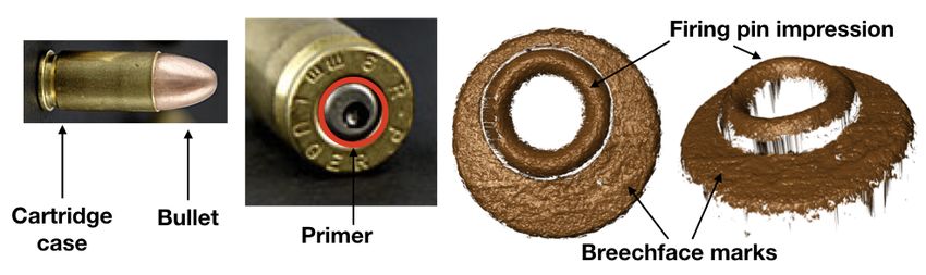
In the case of firearms, firing a gun leaves marks on the bottom surface of the
cartridge case. The mechanism by which this happens is illustrated in Figure 1. Notice
in Figure 1(a) that the bottom surface of the cartridge is in contact with the breech
block of the gun and the firing pin. During the firing process the cartridge is hit by the
firing pin, which causes it to break up into two components: the bullet which goes out
the barrel, and the cartridge case that is ejected from the side. This process leaves at
least two kinds of marks, seen in Figure 1(b). The firing pin hits the cartridge, leaving
a firing pin impression, and the breech block presses against the primer of the cartridge,
leaving breechface marks. The breech block is harder than the primer, and may have
microscopic defects or patterns that are impressed on the primer. This paper focuses
exclusively on breechface marks.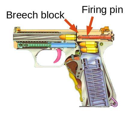
2    William F. Eddy
           Fig. 1: Mechanism by which marks are left on cartridge cases.

(a) Gun that is about (b) On the far left is a cartridge before firing. In the middle left is
to be fired, showing the bottom surface of a cartridge case after firing. On the right are
the internal parts.   images of such a bottom surface, taken using a confocal microscope.
                      The rightmost image shows the image rotated on a horizontal axis.

    Law enforcement officers routinely collect guns and cartridge cases from crime
scenes, because of their potential usefulness in investigations. The Bureau of Alcohol,
Tobacco, Firearms and Explosives (ATF) in the United States maintains a national
database called the National Integrated Ballistics Information Network (NIBIN). This
contains around 3.3 million images of cartridge cases retrieved from crime scenes, and
an additional 12.7 million test fires (as of May 2018) (Bureau of Alcohol, Tobacco,
Firearms and Explosives, 2018). In current practice, cartridge cases may be entered into
NIBIN through a computer-based platform called the Integrated Ballistics Identification
System (IBIS), which was developed and is maintained by Ultra Electronics Forensic
Technology Inc. This platform captures an image of the retrieved cartridge case and
runs a proprietary search against some user-selected subset of the database (for example
images from a certain geographical location). This returns a list of top ranked potential
matches. Firearms examiners may then select a subset that they find to be promising.
They may then locate the physical cartridge cases associated with these images, to
be examined under a comparison microscope. The final determination of a match or
non-match is made by the examiner, based on whether there is “sufficient agreement”
between the marks (AFTE Criteria for Identification Committee, 1992). The examiner
may then bring this evidence to court. It is the examiner that attributes any evidence
to a particular source; the NIBIN system is simply used as an investigative tool to
generate leads. It is up to the discretion of firearms examiners whether or not to enter
retrieved cartridge cases into NIBIN. In addition, the NIBIN database is proprietary
and unavailable for study.
    The current system has been fraught with controversy. Historically, forensic methods
in general have been vetted by the legal system, as opposed to the scientific community.
Beginning in the 1990s, exonerations due to DNA evidence revealed problems in many
forensic science disciplines (Bell et al., 2018). Examiners have been found to have
overstated forensic results, leading (at least in part) to wrongful convictions (Murphy,
2019). A 2009 National Academy of Sciences report (National Research Council, 2009)
called for an overhaul of the forensic science system. With respect to forensic matching,
it stated that with the exception of nuclear DNA analysis, disciplines had neither
scientific support nor a proper quantification of error rates or limitations. In 2016, the
President’s Council of Advisors on Science and Technology (PCAST) followed up with
an independent report (President’s Council of Advisors on Science and Technology,
2016), specifically addressing any scientific developments in the various pattern matching
disciplines. For firearms analysis, there were concerns that there had been insufficient
studies establishing the reliability of conclusions made by examiners, and the associated
Automatically matching topographical measurements of cartridge cases 3
error rates had not been adequately determined. The report suggested two directions
for the future. The first is to “continue to improve firearms analysis as a subjective
method,” by conducting further studies, and the second is to “convert firearms analysis
from a subjective method to an objective method.”
Commercial and academic groups have made some progress with respect to the
second recommendation. For breechface marks, examples of related work include
Song et al. (2018), Roth et al. (2015), Riva and Champod (2014), Thumwarin (2008)
and Geradts et al. (2001). The general methodology is as follows. First select the
relevant breechface marks, using some form of manual input. Then use various image
processing steps to extract relevant features, or derive a similarity score directly. For
example, Song et al. (2018) split the breechface area into a grid of cells and aligns them
independently, producing a similarity score that is defined as the number of matching
cells. A pre-specified cutoff is used for classifying a pair as matched, in other words
coming from the same source. Roth et al. (2015) use a supervised classification method
(gradient boosting) to classify pairs of images as being matched or not. Giudice et al.
(2019) employ a slightly different strategy, developing a fully automatic method that
does not require any pre-processing.
On the commercial side, Ultra Electronics Forensic Technology Inc. maintains the
system used in NIBIN. The software extracts a numerical signature from each region of
interest and does a database search using these signatures (Ultra Electronics Forensic
Technology, 2018). The methodology is proprietary and few details are known. Cadre
Forensics is another manufacturer of microscopes. They extract geometric feature
points that “a trained firearms examiner would identify,” such as ridges, peaks, gouges,
and concavities. These features are then aligned, as a set, to the features from another
image. Logistic regression is used to produce a similarity score, with covariates such as
number of matched features as input (Lilien, 2017).
The shortcomings of currently available methods are that none of them are both
fully automatic and open source. Automatic methods ensure that results are objective
and reproducible, and open source software allows proper testing and validation. In
this paper, we contribute methodology for comparing topographical measurements of
cartridge cases, that is both open source and fully automatic, allowing for a transparent
evaluation. This builds on work in Tai and Eddy (2018), which focuses on reflectance
images as opposed to topographical measurements (more details in Section 2), and Tai
(2018), which proposes a framework for developing forensic matching methods. Software
is available at https://github.com/xhtai/cartridges3D. We apply a record linkage
framework to forensic matching, demonstrating the principled use of statistical methods
in the forensic sciences, at the same time contributing an application of record linkage
methods that is non-traditional. We conduct a comprehensive analysis involving
over 1,100 images, enabling us to compare performance across different firearms and
ammunition. Further, we do a detailed comparison of results produced using older
reflectance microscopy technology versus topographical measurements. All these (and
more; see Section 5) are essential steps before such automated methods can be deployed
in actual criminal cases, or determined to be an improvement over the current system.
At the same time, more work needs to be done to compare the results of automatic
methods to examiner conclusions. If the two are related, results based on automatic
methods might shed some light on examiner error rates over a large number of examples,
and provide insight into comparisons that examiners may struggle with.
The rest of the paper is organized as follows. In Section 2 we first introduce the
data and types of digital representations that are possible with cartridge cases. Section
3 presents the methodology in the context of a record linkage problem. Results are in4 William F. Eddy
Section 4, and Section 5 concludes.
2. Data
Current technology allows for digital representations of fired cartridge cases to be
captured and stored for later comparison. Reflectance microscopes measure the amount
of light reflected off the object’s surface, producing grayscale images. In the literature
these are often called 2D images. Newer technology in the form of 3D profilers (such
as confocal microscopes) measure surface contours directly, producing topographical
measurements. These are often termed 3D images, although both these types of data
come in the form of 2D matrices, with entries being either reflectance or depth values.
For simplicity, in the remainder of this paper we refer to the two types of representations
as 2D and 3D images.
In recent years the National Institute of Standards and Technology (NIST) has
advocated the use of 3D images because of their insensitivity to lighting conditions and
traceability to the International System of Units (SI) unit of length (Song et al., 2012).
The SI system comprises units of measurement built on base units that have precise
standards of measurements. Specifically, base units are derived from invariant constants
of nature (that can be observed and measured with great accuracy), and one physical
artifact. This means that measurements of cartridge cases using any instrument can
be compared to a known standard, and instruments can be calibrated to this known
standard to assess and ensure precision.
The focus of this paper is on developing methods for 3D data. We also compare the
results from comparisons made using 2D and 3D data, to investigate if purportedly
more accurate measurements translate into better comparison results. In the litera-
ture, methods are typically developed for either 2D or 3D data, with limited direct
comparisons made between the two.
We use data from NIST’s Ballistics Toolmark Research Database (https://tsapps.
nist.gov/NRBTD). This is an open-access research database of bullet and cartridge
case toolmark data, which to our knowledge, is the largest publicly available collection
of reference data. Although a national database of firearms data exists (NIBIN), these
data are not publicly available. The NIST database contains images originating from
studies conducted by various groups in the firearm and toolmark community. Almost all
of the currently available data are of cartridge cases that were sent to NIST for imaging,
but the website also allows users to upload their own data in a standardized format.
We study a subset of 1,158 of these images. We limit our analysis to measurements
made by NIST, using disc scanning confocal microscopy. The technology for measuring
surface topographies is relatively new, and as far as we know, there are no standardized
procedures on how these images should be captured. For this paper, we begin with
NIST-collected measurements made using a single method of measurement, for the
sake of uniformity and ease of comparison. Future work could involve examining the
variability due to instrument, method of measurement, and so forth.
The database contains both 2D and 3D images. The various data sets used are
summarized in Table 1, with each data set containing images from a single study.
Among these data are sets involving consecutively manufactured pistol slides, a large
number of firings (termed persistence studies because they investigate the persistence of
marks), as well as a combination of different makes and models of guns and ammunition.
Gun manufacturers include Glock, Hi-Point, Ruger, Sig Sauer, and Smith & Wesson,
and ammunition brands include CCI, Federal, PMC, Remington, Speer, Wolf and
Winchester. Metadata available for download provide additional information such asAutomatically matching topographical measurements of cartridge cases 5
study details, the type of firing pin, material of the primer, etc.
Table 1: Summary of data used from NIST’s Ballistics Toolmark Research Database.
2D and 3D data are available for all studies listed, with the exception of CTS, where
only 3D images exist. Note that for Todd Weller 95 cartridge cases were imaged in 3D
but only 50 were imaged in 2D.
Study Cartridge Firearm Number Slides per Cartridge Test fires per
cases of firearms firearm firearm/slide
Cary Wong 91 Ruger P89 1 1 Winchester 91
CTS 74 Ruger P94DC 1 1 Federal 44
Ruger P91DC 1 1 Federal 18
S&W SW40VE 1 1 Federal 12
De Kinder 70 Sig Sauer P226 10 1 Remington 2
CCI 1
Wolf 1
Winchester 1
Speer 1
Federal 1
Thomas Fadul 40 Ruger P95PR15 1 10 Federal 3-5
Hamby 30 Hi-Point C9 1 10 Remington 3
Kong 36 S&W 10-10 12 1 Fiocchi 3
Laura Lightstone 30 S&W 40VE 1 10 PMC 3
NIST Ballistics 144 Ruger P95D 4 1 Remington 3
Imaging Winchester 3
Database Speer 3
Evaluation PMC 3
(NBIDE) S&W 9VE 4 1 Remington 3
Winchester 3
Speer 3
PMC 3
Sig Sauer P226 4 1 Remington 3
Winchester 3
Speer 3
PMC 3
FBI: Colt 90 Various Colts 45 1 Remington 2
FBI: Glock 90 Various Glocks 45 1 Remington 2
FBI: Ruger 100 Various Rugers 50 1 Remington 2
FBI: S&W 138 Various S&Ws 69 1 Remington 2
FBI: Sig Sauer 130 Various Sig Sauers 65 1 Remington 2
Todd Weller 95 Ruger P95DC 1 10 Winchester 5-9
For the 2D data, each casing was imaged using a Leica FS M reflectance microscope
with ring light illumination. The objective was 2X, the resolution was 2.53 µm, and
images are 1944 × 2592 pixel grayscale files in PNG format. Pixel values range from
0 to 255, where 0 represents black pixels and 255 represents white pixels. 3D data
are measured using a Nanofocus µSurf disc scanning confocal microscope. Various
magnifications were used, for example an objective of 10X results in a lateral resolution
of 3.125µm, and images that are around 1200 × 1200. Pixel values are depth values in
µm (microns).6 William F. Eddy
3. Methodology
3.1. General framework
In order to automatically match 3D images of cartridge cases, we make use of a record
linkage framework. Record linkage is the process of inferring which entries in different
databases correspond to the same real-world identity, in the absence of a unique
identifier (Christen, 2012). Beginning with records from two databases A and B to
be linked, fields such as name and address are pre-processed and standardized. This
results in some set of features for each record. Indexing methods might then be used to
reduce the comparison space, for example candidate pairs in a demographic database
might be restricted to those born in the same month, with all other pairs not being
considered for linkage. Now pairwise comparisons are generated, consisting of one or
more similarity measures. These pairwise data are then classified into matches and
non-matches (and possibly a third category, potential matches). This classification
step may be designed to incorporate restrictions such as one-to-one links, or preserving
transitivity. A clerical review may also be conducted for potential matches, where a
human examines pairs manually to decide the appropriate classification. Finally an
evaluation of the results is conducted.
In Tai (2018), we describe how forensic matching can be thought of as an application
of record linkage; simply think of records as evidence samples, and real-world entity as
the source of the sample. To develop methodology for matching 3D images, we use a
simplified framework illustrated in Figure 2. Each of the steps is described in more
detail in the following subsections.
Fig. 2: Simplified record linkage framework used to develop forensic matching methods.
This is adapted from Tai (2018).
3.2. Features for each record
At an individual record level, the data need to be pre-processed before useful features
can be extracted. Pre-processing typically involves selecting and cleaning up the data
fields. For cartridge cases, each record is an image, so the pre-processing steps are
slightly more involved. The steps we use are 1) Automatically select breechface marks;
2) Level image; 3) Remove circular symmetry; 4) Filter. In Tai and Eddy (2018) we
develop methodology for pre-processing 2D images; methodology for 3D images is
adapted from the former. In Section 4 we compare the results using 2D and 3D data.
Automatically select breechface marks
Looking at Figure 1(b), the area that we are interested in is the area with breechface
marks. We would like to remove all other areas from the analysis, in particular theAutomatically matching topographical measurements of cartridge cases 7
firing pin impression. The breechface region is relatively flat and has a different depth
from the the firing pin impression, since the latter is an indentation on the primer
surface. This is obvious from the rightmost image. The solution that we have adopted
is to fit a plane through the breechface region, ignoring the firing pin impression, and
to select only points lying on or close to the plane.
We use an algorithm called RANdom SAmple Consensus (RANSAC) (Fischler
and Bolles, 1981) to achieve this, and the procedure used is outlined in Algorithm 1.
RANSAC was developed to fit models in the presence of outliers. Briefly, we repeatedly
fit planes to the image by sampling points on the image, and outliers are defined to be
points lying outside some threshold from the fitted plane. The plane with the largest
number of inliers (opposite of outliers) is chosen. These inliers are treated as being
part of the breechface area.
Algorithm 1 RANSAC to find best-fitting plane through Image I
1: procedure bestPlane(I)
2: for i in 1:iter do
3: Sample 3 points from I
4: Fit plane to sampled points
5: Count the number of inliers within preset threshold
6: end for
7: Select model with largest number of inliers
8: Re-fit model using only inliers from selected model
9: return fitted plane, selected inliers
10: end procedure
There are three parameters to be selected: s, the number of points sampled, δ,
the threshold above which points are considered to be outliers, and N , the number
of iterations iter the algorithm runs for (in other words the number of samples). s
is typically the number of points required to fit the model; in this case 3 points are
required to fit a plane. δ = 10µm is selected: Figure 3 shows a typical 3D breechface
image (without a firing pin impression captured) and the associated histogram of depth
values – one can see that most of the depths are within 10µm of each other, making
this a reasonable choice.
Fig. 3: Typical 3D breechface image (without a firing pin impression captured) and
associated histogram of depth values in microns.
As for N , it should be set to be large enough such that the probability of at least
one random sample being free from outliers is at least p. Now, let X be the random8 William F. Eddy
variable denoting the number of samples, out of N , having no outliers. Let e be the
proportion of outliers in the data, and s be the number of sampled points. Then
X ∼ Binom(N, (1 − e)s ), and the goal is to have P[X ≥ 1] ≥ p.
Now, P[X ≥ 1] = 1 − P[X = 0] = 1 − [1 − (1 − e)s ]N , so the objective becomes
1 − [1 − (1 − e)s ]N ≥ p.
Taking logs,
log (1 − p) ≥ N log [1 − (1 − e)s ]
log (1 − p)
N≥
log [1 − (1 − e)s ]
Consider p = .99, s = 3 and e = .6. This last argument says that 60% of points are
outliers. This is set to be a relatively large proportion, since some images capture parts
of the firing pin impression, and all these points would be considered to be outliers.
Nevertheless, e = .6 is still likely to be an overestimate. This gives N ≥ 70. In the
actual implementation we use 75 iterations. Two examples of the resulting breechface
impressions being selected are in Figure 4. Both circular and rectangular firing pin
impressions can be removed well using Algorithm 1. To illustrate further pre-processing
steps, we use the first example in Figure 4.
Fig. 4: Examples of selected breechface areas after applying Algorithm 1. The scale is
in microns. The first set of images is of an example with a circular firing pin impression
and its selected breechface marks, and the second is of an example with a rectangular
firing pin impression.
Level image This step adjusts for the breechface surface being tilted on a plane
during the image capturing process, and has been used in the literature (see e.g.,
Vorburger et al. (2007), Roth et al. (2015)). The same type of tilt in two images could
result in high overall similarity, despite the two having no similar individual features.
This is undesirable since one is less concerned with these overall patterns. To address
this issue, we subtract the plane that was fit in the previous step, planar differences in
depth. The residuals are used for further processing. The first example in Figure 4,
after leveling, is in Figure 5.
Remove circular symmetry Now, we standardize the different resolutions, by
resizing all images to the lowest resolution of 6.25µm. It is at this resolution that
all further pre-processing is done. The next step is to adjust for the surface having
differences in depth that are circular in nature. This adapts the methodology of Tai
and Eddy (2018); here we show that the benefits transfer to topographical data, and
provide the statistical details that were previously omitted. Analogous to the previous
step, the base of the cartridge case could have differences in depth that are circular
in nature. This could arise if the base of the cartridge case slopes inwards towards
the center; looking at the second panel in Figure 1(b), this does look to be the case.Automatically matching topographical measurements of cartridge cases 9
Fig. 5: In Figure 4, the top-left of the first image is shallower than the bottom-right.
This is resolved after leveling the image.
The step of removing circular symmetry corrects for these circular differences in depth,
by fitting a model that captures the differences. The residuals are used for further
processing.
To model the circular differences in depth, we fit a linear combination of circularly
symmetric basis functions (Zeifman, 2014). Consider a square matrix of dimension
m × m, where m is odd. The center entry is at m+1 2 , m+1
2 , and such a matrix is
said to be circularly symmetric if entries located the same distance from the center
entry take the same value. Any matrix can be decomposed into a linear combination of
the matrices in a circularly symmetric basis, plus residuals. The first few matrices in
the basis are shown in Figure 6, where each panel represents one basis matrix. Each
matrix takes the value 1 for pixels that are the same distance from the center, and zero
otherwise. Bases are enumerated from center outwards.
Fig. 6: Illustration of the first eight matrices in a circularly symmetric basis. The
locations in white are the same distance from the center, and matrices are enumerated
from center outwards.
To represent these matrices as basis functions, define functions fk for each matrix
k, taking the ij-coordinates as inputs, and returning the value 0 or 1 depending on
whether the input location is the required distance, dk , from the center, i.e., if it is white
or black in the pictorial representation in Figure 6. An example of a basis function (the
fifth one, enumerated from the center outwards) is in Equation 1. The decomposition
of a matrix can then be represented as Equation 2, where K is the number of basis
functions, fk is the kth basis function, βk is the basis function coefficient for fk , and
is the error.
( √
1 if d(i, j) = d5 = 5
f5 (i, j) = (1)
0 otherwise.10 William F. Eddy
K
X
Image(i, j) = βk fk (i, j) + (i, j) (2)
k=1
The number of basis functions required, K, depends on the resolution of the image.
For example, a 3 × 3 image has three possible distances from the center (including
the corners), and can be represented using three basis functions. A 701 × 701 image
(this is the size of the NIST 3D images after cropping and standardizing resolutions)
requires 39,978 basis functions. The coefficient for each basis function is the mean of
pixel values for pixels with the corresponding distance from the center.
In this analysis missing pixels are ignored. Since only the breechface marks are
selected for analysis, treating the other regions as missing pixels, some fraction of the
coefficients will not be computed, but the total number of coefficients is still very large.
There are large local fluctuations in the model coefficients since many of them are
estimated only using a small number of pixels (many basis functions only have four
pixels, and many of the pixels are also missing due to the selection of the breechface
area). In order to only capture a global effect, a loess regression (Cleveland, 1979) is fit
to the basis coefficients to reduce the variance of the estimates.
Loess regression assumes that yi = f (xi ) + i , where i is the error. The function f is
approximated at each point in the range of the data set, using a low-degree polynomial
and weighted least squares. Weights are inversely proportional to the distance from the
point of interest. The parameters required for estimating the function are the degree of
the polynomial, the weighting function, and the proportion of all points to be included
in the fit. Here a quadratic function is fit, and the proportion of points to be included
in the fit is set to be α = 0.75. The weight function (for local points that are included)
3 3
from the point x0 is computed using a tricubic kernel wi (x0 ) = 1 − |xih−x 0
0|
, where
h0 is the (α ∗ n)th largest |xi − x0 |. A large value of α was selected for a large degree of
smoothing, as can be seen in Figure 7(a). With this large degree of smoothing, the loess
regression is not particularly sensitive to the weight function or degree of polynomial,
and we simply used the default values implemented in the loess() function in R.
Loess regression is a linear smoother, meaning that the fitted values are a linear
combination of the original values (Buja et al., 1989). Precisely, Ŷ = SY, where S is
an n × n matrix, called a smoother matrix. The smoother matrix is analogous to the
hat matrix in multiple linear regression: Ŷ = HY, where H = X(XT X)−1 XT Y. The
trace of the smoother matrix is the effective degrees of freedom of the loess regression,
and using these specifications the effective degrees of freedom is less than 5 for each
image. Results for the same example image are in Figure 7. There is evidence of an
inward slope towards the center, which we hypothesized based on Figure 1(b).
The fitted model and the residuals for the same example image are in Figure 7. The
two identified sources of bias, planar and circular, are no longer present in the residuals.
Filter The last pre-processing step is filtering, which again has been used in the
literature. Filtering highlights certain features of the image. A Gaussian filter is used,
with short and long cutoffs approximately 20-150µm, meaning that patterns with
wavelengths within this range are highlighted. Empirically these produced the best
results among some test examples; as far as we know there is no established guidance
on what wavelengths are relevant for the comparison. Some cutoffs that have been
used in other work are 2.5-250µm, 37-150µm (Vorburger et al., 2007), and 16-250µm
(Song et al., 2018).
The resulting image after all pre-processing is on the left in Figure 8. Note the
prominence of marks compared to the original image in the left panel of Figure 4.Automatically matching topographical measurements of cartridge cases 11
Fig. 7: Removing circular symmetry from the example image.
(a) The set of circularly symmetric basis functions is fit (b) Residual image produced.
to the example residual image after leveling (Figure 5).
3.3. Pairwise comparison: Similarity for each pair of records
Given features for individual records, the next step is to generate meaningful similarity
scores for pairwise comparisons. In this particular application, it is necessary to first
align the two images to one another. Aligning images typically involves finding the
best rotation and translation parameters (horizontal and vertical), where “best” means
some metric is optimized, over all pixels or some subset of pixels. This optimization
can be done either using a grid search or some other approximate means. The metric
used might be correlation, mean-squared error, or something similar. Frequently, the
optimized value of the metric is used as a similarity measure; this might be used on its
own or combined with other similarity measures to produce a feature set for comparing
two images.
In the literature, perhaps the most widely used measure of similarity is the maximized
correlation over rotations and translations, known as CCFmax , or maximum cross-
correlation function (see e.g., Vorburger et al., 2007; Roth et al., 2015; Riva and
Champod, 2014; Geradts et al., 2001). This is what we use here. To be precise,
the cross-correlation between two zero-mean images I1 and I2 (or more generally,
2-dimensional matrices), is defined as
P
i,j I1 (i, j)I2 (i + k, j + l)
CCFI1 ,I2 (k, l) = qP qP , (3)
(i, 2 2
I
i,j 1 j) i,j I2 (i, j)
where (k, l) represents spatial lag (translation; with k and l being the vertical and
horizontal lags respectively), i indexes the rows and j indexes the columns. The
computation is repeated for different rotation angles, and CCFmax is then the maximum
correlation, taking into account rotations and translations.
We use a grid search to maximize the correlation between two images over translations
and rotations. The maximized correlation derived in this manner is an estimator of
CCFmax , or more precisely, CCFImax 1 ,I2
, where the two images being compared are I1
and I2 . The details are in Algorithm 2.
Let the correlation returned by Algorithm 2 be cˆ12 . Now, for a comparison of I1
and I2 , one can either align I2 to I1 using align(I1 , I2 ) to return cˆ12 , or I1 to I2
using align(I2 , I1 ) to return cˆ21 . This might give slightly different results due to
computational issues such as interpolation that is involved during a rotation. We12 William F. Eddy
Algorithm 2 Aligning image 2 to image 1
1: procedure align(I1 , I2 )
2: thetas ← −175, −170, .P . . , −10, −7.5, −5, . . . , 5, 7.5, 10, 15, . . . , 180
3: Scale I1 (so I¯1 = 0 and ij I1 (i, j)2 = 1) . So that maximizing correlation ≡
minimizing MSE
4: for theta in thetas do
5: Rotate I2 by theta
6: Scale rotated I2
7: Compute cross-correlation, CCFIθ1 ,I2 (k, l), as in Equation 3, for integer k
and l
8: CCFIθ1 ,I2 ← maxk,l CCFI1 ,I2 (k, l)
9: end for
10: θ0 ← arg maxθ CCFIθ1 ,I2 . Neighborhood of best θ
11: 0
if θ ∈ [−10, 10] then
12: fineThetas ← θ0 − 2, θ0 − 1.5, . . . θ0 + 2
13: else
14: fineThetas ← θ0 − 4, θ0 − 3, . . . θ0 + 4
15: end if
16: for theta in fineThetas do . Finer search in neighborhood of θ0
17: Lines 5-8
18: end for
0
19: θ? , kθ? , lθ? ← arg maxθ0 CCFIθ1 ,I2
0
20: CCFImax 1 ,I2
← maxθ0 CCFIθ1 ,I2
21: return CCFImax 1 ,I2
, θ? , kθ? , lθ?
22: end procedure
compare cˆ12 to cˆ21 for each of the data sets, and note that the differences are minimal.
We define the similarity score between two images to be
sˆ12 = max(cˆ12 , cˆ21 )
(4)
= max(align(I1 , I2 ), align(I2 , I1 )),
and this single pairwise feature is used for classification.
To illustrate the results, Algorithm 2 is applied to a pair of example images in
Figure 8, where both are from the same gun. A similarity score of 0.76 is obtained,
with a rotation angle of 13◦ , meaning that the second image is rotated 13◦ clockwise
for best alignment. Plotting the two images with the second rotated, notice that the
breechface marks are now lined up well.
3.4. Classification
After pairwise similarity scores have been generated, there are numerous methods to
classify the pairs into predicted matches and non-matches. We use a threshold-based
approach, meaning that cutoffs on ŝ can be used, above which pairs are classified as
matches. The effects of choosing various cutoffs are examined using precision-recall
graphs (see 3.6).Automatically matching topographical measurements of cartridge cases 13
Fig. 8: The example image from the previous figures is on the left. On the right is a
processed image from the same gun, after alignment. Note that the parallel marks are
now lined up well.
3.5. Hierarchical clustering
In record linkage, additional restrictions are sometimes imposed in the matching process.
For example, a one-to-one constraint may be added, meaning that a record in database
A can be matched to only one record in database B. Another common situation is when
multiple pairwise comparisons are done independently, and there is a desire to eliminate
intransitive links. For example, if A matches B and B matches C, but A does not match
C, there is a conflict that needs to be resolved. Here we use hierarchical clustering to
eliminate intransitive links, in situations where these intransitive links are undesirable.
For example, we might be interested in comparing results of an automatic method with
that of examiner proficiency tests. In these tests multiple samples from test fires using
the reference firearm are provided as reference samples. Examiners need to determine
if various questioned samples come from the same source as the reference samples.
Essentially, this involves organizing samples into groups that examiners believe come
from the same source. These are necessarily transitive in terms of pairwise comparisons,
and is arguably a simpler task than getting each pairwise comparison correct. To
compare these results accurately with results from an automated method would require
that the latter also have transitive links. Additionally, reference data sets are often
used in developing automated methods. Researchers perform all pairwise comparisons
within these data sets, and if there are intransitive links there would be inconsistencies
in the evaluation. A final argument for imposing the constraint of transitivity is that it
can lead to better classifier performance.
As far as we know, the issue of intransitivity has not been seriously considered in the
forensic matching literature. It is possible that it is not a concern depending on the goals
of the analysis, but we argue for its inclusion as an optional post-processing step. We
adopt the approach in Ventura et al. (2015), where given pairwise similarity predictions
s, we use d = 1 − s as a distance measure, and perform hierarchical agglomerative
clustering using various linkage methods.
Briefly, given items 1, . . . , n, dissimilarities dij between each pair i and j, and
dissimilarities d(G, H) between groups G = {i1 , i2 , . . . ir } and H = {j1 , j2 , . . . , js },
hierarchical agglomerative clustering starts with each node in a single group, and
repeatedly merges groups such that d(G, H) is within a threshold D. d(G, H) is
determined by the linkage method, and here we use single, complete, average (Everitt
et al., 2001) and minimax linkage (Bien and Tibshirani, 2011). These linkage methods
define d(G, H), as follows.
Single linkage dsingle (G, H) = mini∈G,j∈H dij14 William F. Eddy
Complete linkage dcomplete (G, H) = maxi∈G,j∈H dij
1 P
Average linkage daverage (G, H) = |G||H| i∈G,j∈H dij
Minimax linkage dminimax (G, H) = mini∈G∪H r(i, G ∪ H), where r(i, G) =
maxj∈G dij , the radius of a group of nodes G around i
Employing a linkage method and making a choice of cutoff would result in a data
set that is grouped into clusters that share the same source.
3.6. Evaluation
The classification step generates predictions for whether pairs are matches or non-
matches (depending on some cutoff). Similarly, after hierarchical clustering the com-
parisons can be evaluated on a pairwise level. Since the metadata provided in NIST’s
database gives information on the source of each image, ground truth labels for whether
pairs are from the same gun (a match or non-match) can be generated. One can use
the same performance measures used in classification problems, at a pairwise level.
In the forensics literature, evaluation on reference data is done in a haphazard
manner. Most commonly, plots of score distributions from true matched and non-
matched pairs are displayed as histograms (Vorburger et al., 2007; Ott et al., 2017;
Song et al., 2018; Roth et al., 2015; Riva and Champod, 2014; Lilien, 2017), and a
comment is made based on the visual separation between the distributions. If there
is good separation between scores for matched and non-matched pairs, the method is
said to be successful. Other work estimates the overlapping area between distributions,
or the number of true matches in among the top 10 pairs in terms of similarity scores
(Vorburger et al., 2007). Some other examples are the mean and standard deviation of
the distributions of scores for matched and non-matched pairs (Ott et al., 2017), false
positive and false negative rates, false discovery and false omission rates (Song et al.,
2018), and ROC curves (Roth et al., 2015).
We propose standardizing the evaluation process by reporting precision and recall,
as well as the area under the precision-recall graph as a numerical summary. This gives
a better characterization of classifier performance, as opposed to visually comparing the
two distributions. It is also an improvement over estimating the overlap region, since
the latter often requires assumptions to be made about the data. It is more informative
than other summary measures like mean and standard deviation of the distributions.
The choice of precision and recall is explained as follows. A typical confusion matrix
in a classification problem has the following cells:
Predicted
Truth 0 1
0 True Negative False Positive
1 False Negative True Positive
In record linkage problems, there is a large class imbalance since most pairs do not
match, so typically, pairs are overwhelmingly true negatives. Measures that have the
number of true negatives in the denominator, such as false positive rate, will often
True Positives
be close to zero. Hence we propose using Precision = True Positives + False Positives and
True Positives
Recall = True Positives + False Negatives . Both measures range from 0 to 1, with 1 being
perfect classifier performance.
Since in our case the cutoff for predicting positives (matches) is not necessarily fixed
(more details in Section 4.1.2), we compute the area under the precision-recall graph.Automatically matching topographical measurements of cartridge cases 15
This also ranges from 0 to 1, and maximum performance is achieved when the graph
passes through the top-right corner, giving an area under the curve of 1.
4. Results
We first present results of our proposed methodology in Section 4.1, followed by
comparisons between 3D and 2D data.
4.1. 3D results
4.1.1. Classifier and clustering accuracy
For each data set described in Table 1, we run the complete pipeline as described
in Section 3. We perform all pairwise comparisons for each data set, evaluating the
results both after the classification step and after the hierarchical clustering step. We
first present distributions of similarity scores ŝ for true matches and non-matches by
data set in Figure 9. We then look at precision-recall graphs in Figure 10, with lines
representing results both before and after hierarchical clustering.
The results are organized by type of data set. Of the 14 data sets studied, four involve
consecutively manufactured pistol slides firing the same ammunition. The pistol slide
is a component of the firearm that includes the breech block, and is hence responsible
for the breechface marks. It had been suggested that pistol slides that were produced
successively might have similar patterns and imperfections that persist through the
manufacturing process (see e.g., Lightstone, 2010), so cartridge cases obtained using
such slides might be more difficult to differentiate. Lightstone (2010) found that firearms
examiners did not in fact have trouble comparing such cartridge cases, because even
though the molds that were used to produce the slides did have markings that carried
over through the manufacturing process, the individual characteristics on each slide
were sufficient for examiners to make correct identifications to the individual slide. Here
one can come to the same conclusion: in Figures 9(a) to 9(d) the method produces
higher similarity scores for most comparisons belonging to the same pistol slide, than
those involving different slides. All the plots show a very good separation between the
true match and non-match distributions. At least for the combinations of firearm and
ammunition studied, having pistol slides that are consecutively manufactured does not
appear to pose a problem for automatic identification.
Now consider the Kong and De Kinder data sets, which involve multiple copies of the
same firearm. Kong uses 12 Smith & Wesson 10-10’s, firing Fiocchi ammunition. One
might expect results to mimic those that involve consecutively manufactured slides, but
this does not turn out to be the case; results are far worse. De Kinder on the other hand,
uses 10 Sig Sauer P226’s, firing six different brands of ammunition, and the results also
show extremely poor separation between match and non-match scores. From the Kong
study, manually looking at examples of non-matched pairs producing very high scores
(over .6), one observation is that the markings appear as small scratches, and are very
much less pronounced compared to those in Figure 1(b), say. It has been noted by
firearms examiners that some guns mark more poorly than others, leading to difficult
comparisons, and this could be an example of this phenomenon.
Next, results for the NBIDE, CTS and FBI data sets are in Figures 9(g) to 9(m).
These all involve either multiple ammunition or firearm types. The five FBI data
sets use various Colts, Glocks, Rugers, Sig Sauers and Smith & Wessons, and only
Remington ammunition, while CTS uses Rugers and Smith & Wesson firearms and
Federal ammunition. NBIDE uses different firearms with Remington, Winchester, Speer
and PMC ammunition. For all these data sets, there is a range of separation between16 William F. Eddy
the match and non-match scores. Gun brands that have the best performance look to
be Glock, Ruger and Smith & Wesson.
Finally, the Cary Wong data set involves a single type of firearm (Ruger P89) and
ammunition (Winchester), but the gun is fired 2000 times. Cartridge cases 25-1000
at intervals of 25 test fires are imaged, as well as the first 10 and the 1001st test fire,
giving a total of 91 images. The purpose of this study was to investigate if marks
persisted over multiple fires, say, over the lifespan of a gun that is heavily used. The
results in show a range of ŝ values. This suggests that we may be able to identify some
but not all cartridge cases to this particular firearm, in its entire lifespan.
Precision-recall graphs before and after clustering are in Figure 10. Note that the
Cary Wong data set is excluded from this presentation because there are no non-matched
pairs in this data set. The results in Figure 10 corroborate the visual findings presented
in Figure 9, and provide a convenient numerical summary of performance. We find that
the clustering step results in better AUCs for data sets that are not at the extremes
in terms of performance (either very poor or close to perfect): the larger differences
are for Hamby (.87 to .93), NBIDE (.86 to .94), CTS (.87 to .94), FBI Colt (.6 to .64).
Overall, very good performance is achieved in 9 of the 13 data sets, where AUCs are
over .9 using at least one linkage method. One might hypothesize as to why clustering
improves performances. Minimax linkage, for example, selects a cluster center for each
cluster, and members of the cluster need to be similar to this center but not necessarily
to other members of the cluster. It is plausible that the cluster center is a particularly
well-marked cartridge case, while other cluster members might have areas that are less
well-marked.
We have so far been agnostic about the selection of a similarity cutoff to designate
predicted matches and non-matches. This might be of interest in some situations. For
example, one might be interested in selecting pairs above a cutoff for further manual
investigation. Alternatively, a cutoff could be used to make a conclusion in criminal
cases on whether a person should be implicated in a crime. The choice of cutoff depends
on the goal and desired tradeoff between false negatives and false positives. In the first
investigative case a lower cutoff might be set to ensure high recall, while in the second
case a much higher cutoff might be necessary, since the costs associated with falsely
implicating a suspect are disproportionately high.
4.1.2. Final clusters
Suppose that for comparison with examiner proficiency tests, we are interested in
producing a disambiguated data set where images are clustered based on whether they
share a common source. This requires the selection of a cutoff as well as a linkage
method. Figure 10 shows the range of values of precision and recall that can be achieved
using various cutoffs and different linkage methods. For the purposes of illustration we
treat false negatives and false positives equally, and choose a cutoff that maximizes
precision and recall; this corresponds to the value at the bend of the precision-recall
curve. As for the linkage method, examining results from the different data sets, it
appears that minimax and average linkage have good performance across the board. In
addition, minimax linkage has the advantage of being interpretable, so minimax linkage
is selected to generate final clusters. Using minimax linkage, a cutoff that works well
for all data sets is around .4, so we select this value.
We illustrate the results using the NBIDE data set; one can repeat this analysis for
any data set. The NBIDE data set consists of a total of 144 images from 12 different
guns. If the algorithm worked perfectly, one would expect to see 12 clusters of size 12.
Instead, the cluster sizes are shown in Table 2. Now, comparing to ground truth, all 6Automatically matching topographical measurements of cartridge cases 17
clusters of 12 are correct, and correspond to 4 Ruger firearms, and 2 Sig Sauers. The
remaining 6 firearms comprise of combining two or more of the smaller clusters, with
one exception: one cluster of size 4 mistakenly puts a cartridge case from a Smith &
Wesson firearm in a cluster containing cartridge cases from a different Smith & Wesson
firearm. In terms of performance by gun brand, it appears that from best to worst are
Ruger, Sig Sauer, and then Smith & Wesson.
Table 2: Cluster sizes for the NBIDE data set in 3D, after hierarchical clustering using
minimax linkage with a cutoff of .4. Perfect results would be 12 clusters of size 12.
Cluster Size 1 3 4 5 6 7 9 12
Count 2 5 4 1 3 1 1 6
4.2. Comparison between 2D and 3D
In Section 2 we explained the two types of technology currently available for producing
digital representations of the data: 2D reflectance images, and 3D topographical
measurements. We mentioned that NIST has advocated for the use of 3D topographies.
In this section we investigate how the individual pairwise comparison results differ for
the two types of images, to investigate if the 3D representation does indeed produce
superior results. The results presented in Section 4.1 involve 14 different data sets. The
same data are available in 2D, with the exception of CTS and Todd Weller. CTS data
are completely unavailable in 2D, while a subset of 50 out of the 95 Weller images are
available in 2D. All available data are used for comparing the two different types of
data.
For processing 2D images, we use methodology from Tai and Eddy (2018). Full
details are in the paper; the main differences are that for 2D data we used edge detection
and image processing operations to select the breechface marks, whereas in 3D, we
make use of differences in depth measurements. Processing 2D data also involves the
additional step of removing outliers. The resolution used for comparisons in 2D was
10µm, compared to 25µm for 3D topographies.
The individual correspondences of 2D and 3D scores for each pairwise comparison
is in Figure 11. We notice that there is no straightforward correspondence between the
scores, and it is not uniformly the case that results in 3D are superior. For some of
the consecutively manufactured data sets for example, the separation in match and
non-match score distributions is actually better in 2D than in 3D. It is true in general
however, that 3D produces better performance. 3D scores are generally higher than 2D
scores, and high 2D scores generally correspond to high 3D scores. If the 2D score is low
however, 3D scores span the entire range of values. For non-matches this is undesirable,
but for matches the opposite is true, resulting in the overall better performance using
3D images.
5. Discussion and conclusion
In this paper, we develop methodology to match topographical measurements of
cartridge cases. This methodology is both fully automatic and open source, and we
evaluate it comprehensively on over 1,100 publicly-available images. We compare results
to that using older reflectance microscopy images.
We make several specific improvements over existing methods. First, the selection
of breechface marks is automated using RANdom SAmple Consensus (RANSAC).
Removing circular symmetry during pre-processing removes artifacts like the slope18 William F. Eddy
of the primer surface downwards towards the center. This reduces the likelihood of
spurious correlations. We standardize evaluation using precision-recall graphs, and
attach a numerical summary by reporting the area under the curve. Finally, resolving
intransitive links and generating a linked data set has not been given much thought
in the forensics literature, and we propose ways to address this using ideas from the
record linkage literature. We contribute a non-traditional application of record linkage.
Several domain-specific conclusions that are of interest are that performance using
topographical measurements have better overall performance than reflectance images
over a large number of data sets, but individual comparisons vary in quality. Excellent
overall performance is achieved (area under the precision-recall curve of over .9) in
9 out of the 13 data sets studied. Performing the clustering step generally improved
performance, particularly for data sets with middling to good (but not excellent) results.
Performance is generally good on consecutively manufactured data sets, whereas other
types of data sets could have much poorer performance. It is not possible to make
general statements about particular gun or ammunition brands, since there is a lot of
variability depending on the gun model and data collection effort. One clear conclusion
from the variety of data sets analyzed, is that some specific firearm and ammunition
combinations produce far superior results than others. More work needs to be done to
investigate and explain these differences.
There are at least two specific directions of future work that are essential if such
methods are to be adopted for use in actual criminal cases. The first is to do a much
more comprehensive comparison of the results of automatic methods with that of
human examiners. There is some evidence to suggest that examiner performance might
be related to algorithmic performance; for example, Lightstone (2010) concludes that
examiners did not have difficulty differentiating consecutively manufactured slides, and
in this paper neither does an automatic method. Much more work needs to be done
before reaching a definitive conclusion, but establishing a relationship between examiner
and algorithmic performance would be beneficial in many ways. For example, data on
examiner error rates are generally lacking, and results using automatic methods may
serve as a guide to examiner error rates. Types of comparisons that are problematic
for algorithms could suggest problems for examiners as well. The second issue is to
examine the fairness of automatic methods. As such methods have risen in popularity in
forensic matching, there have been calls from government to consider this issue (Takano,
2019). In firearms matching, we have already seen large differences in performance
depending on the data set studied. The first step would be do a proper accounting
of these differences. Next and more importantly, is to examine if these translate into
bias towards any particular group, for example through geography, or different costs of
guns and ammunition resulting in different groups favoring certain types of guns or
ammunition.
To conclude, automatic methods have a lot of potential in terms of corroborating,
enhancing, and possibly one day replacing examiner testimony. We have produced good
results on many data sets, but these methods need to be tested much more extensively
before being used in real cases, where there is the possibility of unintended harms, and
where the consequences of falsely implicating a suspect are severe.
References
AFTE Criteria for Identification Committee
1992. Theory of identification, range of striae comparison reports, and modifiedAutomatically matching topographical measurements of cartridge cases 19 glossary definitions – an AFTE criteria for identification committee report. AFTE Journal, 24(2):336–340. Bell, S., S. Sah, T. D. Albright, S. J. Gates, M. B. Denton, and A. Casadevall 2018. A call for more science in forensic science. Proceedings of the National Academy of Sciences, 115(18):4541–4544. Bien, J. and R. Tibshirani 2011. Hierarchical clustering with prototypes via minimax linkage. Journal of the American Statistical Association, 106 495:1075–1084. Buja, A., T. Hastie, and R. Tibshirani 1989. Linear smoothers and additive models. The Annals of Statistics, 17(2):453–510. Bureau of Alcohol, Tobacco, Firearms and Explosives 2018. Fact sheet - national integrated ballistic information network. Christen, P. 2012. Data Matching: Concepts and Techniques for Record Linkage, Entity Resolu- tion, and Duplicate Detection. Springer Publishing Company, Incorporated. Cleveland, W. S. 1979. Robust locally weighted regression and smoothing scatterplots. Journal of the American Statistical Association, 74(368):829–836. Everitt, B., S. Landau, and M. Leese 2001. Cluster analysis, 4th edn: Arnold. London, UK. Fischler, M. A. and R. C. Bolles 1981. Random sample consensus: A paradigm for model fitting with applications to image analysis and automated cartography. Commun. ACM, 24(6):381–395. Geradts, Z. J., J. Bijhold, R. Hermsen, and F. Murtagh 2001. Image matching algorithms for breech face marks and firing pins in a database of spent cartridge cases of firearms. Forensic Science International, 119(1):97–106. Giudice, O., L. Guarnera, A. B. Paratore, G. M. Farinella, and S. Battiato 2019. Siamese ballistics neural network. In 2019 IEEE International Conference on Image Processing (ICIP), Pp. 4045–4049. Lightstone, L. 2010. The potential for and persistence of subclass characteristics on the breech faces of SW40VE Smith & Wesson Sigma pistols. AFTE Journal, 42(4):308–322. Lilien, R. 2017. Applied research and development of a three-dimensional topography system for imaging and analysis of striated and impressed tool marks for firearm identification using gelsight. Forensic Science Seminar, 7(2):43–53. Murphy, H. 2019. A leading cause for wrongful convictions: Experts over- stating forensic results. https://www.nytimes.com/2019/04/20/us/ wrongful-convictions-forensic-results.html, accessed: 2019-04-28. National Research Council 2009. Strengthening Forensic Science in the United States: A Path Forward. Wash- ington, DC: The National Academies Press. Ott, D., R. Thompson, and J. Song 2017. Applying 3D measurements and computer matching algorithms to two firearm examination proficiency tests. Forensic Science International, 271:98 – 106. President’s Council of Advisors on Science and Technology 2016. Report to the President on Forensic Science in Criminal Courts: Ensuring Scientific Validity of Feature-Comparison Methods. Washington, D.C.: Executive Office of the President.
You can also read